Work in progress.
In this notebook, we explore how surrogate gradient descent solves the sound localisation problem when restricted to using only excitatory connections.
We use the spiking solution provided in the last section of the Starting Network and we force W1 (input to hidden layer) and W2 (hidden to output layer) to be positive. We reason that this might constrain the learning to a more classical coincidence-detector strategy on the hidden layer. It is also more biologically relevant since neurons often have an excitatory or inhibitory effect on their partners but not both (known as Dale’s law).
import numpy as np
import matplotlib.pyplot as plt
import matplotlib.colors
import matplotlib.cm

import torch
import torch.nn as nn

!pip install tqdm
from tqdm.auto import tqdm as pbar

dtype = torch.float

if torch.cuda.is_available():
    device = torch.device("cuda")
else:
    device = torch.device("cpu")
Requirement already satisfied: tqdm in /home/riquelmej/opt/anaconda3/envs/spikeloc/lib/python3.10/site-packages (4.64.0)
# Constants
SECONDS = 1
MS = 1e-3
HZ = 1

DT = 1 * MS            # large time step to make simulations run faster
ANF_PER_EAR = 100    # repeats of each ear with independent noise

DURATION = .1 * SECONDS # stimulus duration
DURATION_STEPS = int(np.round(DURATION / DT))
INPUT_SIZE = 2 * ANF_PER_EAR
def input_signal(ipd):
"""
Generate an input signal (spike array) from array of true IPDs
"""
envelope_power = 2 # higher values make sharper envelopes, easier
rate_max = 600 * HZ # maximum Poisson firing rate
stimulus_frequency = 20 * HZ
num_samples = len(ipd)
times = np.arange(DURATION_STEPS) * DT # array of times
phi = 2*np.pi*(stimulus_frequency * times + np.random.rand()) # array of phases corresponding to those times with random offset
# each point in the array will have a different phase based on which ear it is
# and its delay
theta = np.zeros((num_samples, DURATION_STEPS, 2*ANF_PER_EAR))
# for each ear, we have anf_per_ear different phase delays from to pi/2 so
# that the differences between the two ears can cover the full range from -pi/2 to pi/2
phase_delays = np.linspace(0, np.pi/2, ANF_PER_EAR)
# now we set up these theta to implement that. Some numpy vectorisation logic here which looks a little weird,
# but implements the idea in the text above.
theta[:, :, :ANF_PER_EAR] = phi[np.newaxis, :, np.newaxis]+phase_delays[np.newaxis, np.newaxis, :]
theta[:, :, ANF_PER_EAR:] = phi[np.newaxis, :, np.newaxis]+phase_delays[np.newaxis, np.newaxis, :]+ipd[:, np.newaxis, np.newaxis]
# now generate Poisson spikes at the given firing rate as in the previous notebook
spikes = np.random.rand(num_samples, DURATION_STEPS, 2*ANF_PER_EAR)<rate_max*DT*(0.5*(1+np.sin(theta)))**envelope_power
return spikes
def random_ipd_input_signal(num_samples, tensor=True):
"""
Generate the training data
Returns true IPDs from U(-pi/2, pi/2) and corresponding spike arrays
"""
ipd = np.random.rand(num_samples)*np.pi-np.pi/2 # uniformly random in (-pi/2, pi/2)
spikes = spikes_from_fixed_idp_input_signal(ipd, tensor)
if tensor:
ipd = torch.tensor(ipd, device=device, dtype=dtype)
return ipd, spikes
def spikes_from_fixed_idp_input_signal(ipd, tensor=True):
spikes = input_signal(ipd)
if tensor:
spikes = torch.tensor(spikes, device=device, dtype=dtype)
return spikes
def show_examples(shown=8):
ipd = np.linspace(-np.pi/2, np.pi/2, shown)
spikes = spikes_from_fixed_idp_input_signal(ipd, shown)
plt.figure(figsize=(10, 4), dpi=100)
for i in range(shown):
plt.subplot(2, shown // 2, i+1)
plt.imshow(spikes[i, :, :].T, aspect='auto', interpolation='nearest', cmap=plt.cm.gray_r)
plt.title(f'True IPD = {int(ipd[i]*180/np.pi)} deg')
if i>=4:
plt.xlabel('Time (steps)')
if i%4==0:
plt.ylabel('Input neuron index')
plt.tight_layout()
show_examples()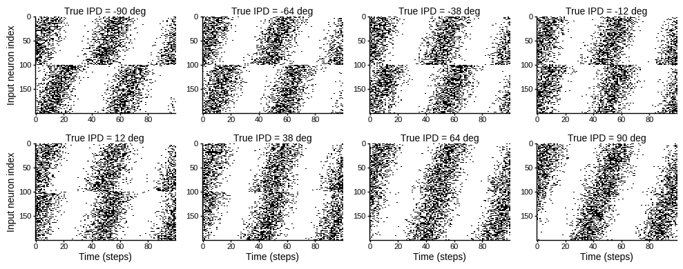
Setup training hyper parameters
my_computer_is_slow = True # set this to True if using Colab

N_EPOCHS = 50

# Parameters for training. These aren't optimal, but instead designed
# to give a reasonable result in a small amount of time for the tutorial!
if my_computer_is_slow:
    batch_size = 64
    n_training_batches = 64
else:
    batch_size = 128
    n_training_batches = 128
n_testing_batches = 32
num_samples = batch_size*n_training_batches
# Generator function iterates over the data in batches
# We randomly permute the order of the data to improve learning
def data_generator(ipds, spikes):
    perm = torch.randperm(spikes.shape[0])
    spikes = spikes[perm, :, :]
    ipds = ipds[perm]
    n, _, _ = spikes.shape
    n_batch = n//batch_size
    for i in range(n_batch):
        x_local = spikes[i*batch_size:(i+1)*batch_size, :, :]
        y_local = ipds[i*batch_size:(i+1)*batch_size]
        yield x_local, y_local

def test_accuracy(ipds, spikes, run):
    accs = []
    ipd_true = []
    ipd_est = []
    confusion = np.zeros((NUM_CLASSES, NUM_CLASSES))
    for x_local, y_local in data_generator(ipds, spikes):
        y_local_orig = y_local
        y_local = discretise(y_local)
        output = run(x_local)
        m = torch.sum(output, 1)  # Sum time dimension
        _, am = torch.max(m, 1)  # argmax over output units
        tmp = np.mean((y_local == am).detach().cpu().numpy())  # compare to labels
        for i, j in zip(y_local.detach().cpu().numpy(), am.detach().cpu().numpy()):
            confusion[j, i] += 1
        ipd_true.append(y_local_orig)
        ipd_est.append(continuise(am.detach().cpu().numpy()))
        accs.append(tmp)
    ipd_true = np.hstack(ipd_true)
    ipd_est = np.hstack(ipd_est)

    return ipd_true, ipd_est, confusion, accs

def report_accuracy(ipd_true, ipd_est, confusion, accs, label):

    abs_errors_deg = abs(ipd_true-ipd_est)*180/np.pi

    print()
    print(f"{label} classifier accuracy: {100*np.mean(accs):.1f}%")
    print(f"{label} absolute error: {np.mean(abs_errors_deg):.1f} deg")

    plt.figure(figsize=(10, 4), dpi=100)
    plt.subplot(121)
    plt.hist(ipd_true * 180 / np.pi, bins=NUM_CLASSES, label='True')
    plt.hist(ipd_est * 180 / np.pi, bins=NUM_CLASSES, label='Estimated')
    plt.xlabel("IPD")
    plt.yticks([])
    plt.legend(loc='best')
    plt.title(label)
    plt.subplot(122)
    confusion /= np.sum(confusion, axis=0)[np.newaxis, :]
    plt.imshow(confusion, interpolation='nearest', aspect='equal', origin='lower', extent=(-90, 90, -90, 90))
    plt.xlabel('True IPD')
    plt.ylabel('Estimated IPD')
    plt.title('Confusion matrix')
    plt.tight_layout()


def analyse_accuracy(ipds, spikes, run, label):
    ipd_true, ipd_est, confusion, accs = test_accuracy(ipds, spikes, run)
    report_accuracy(ipd_true, ipd_est, confusion, accs, label)
# classes at 15 degree increments
NUM_CLASSES = 180 // 15
print(f'Number of classes = {NUM_CLASSES}')

NUM_HIDDEN = 30

def discretise(ipds):
    return ((ipds+np.pi/2) * NUM_CLASSES / np.pi).long() # assumes input is tensor

def continuise(ipd_indices): # convert indices back to IPD midpoints
    return (ipd_indices+0.5) / NUM_CLASSES * np.pi - np.pi / 2
Number of classes = 12
def sigmoid(x, beta):
    return 1 / (1 + np.exp(-beta*x))

def sigmoid_deriv(x, beta):
    s = sigmoid(x, beta)
    return beta * s * (1 - s)


# noinspection PyAbstractClass,PyMethodOverriding
class SurrGradSpike(torch.autograd.Function):
    @staticmethod
    def forward(ctx, inp):
        ctx.save_for_backward(inp)
        out = torch.zeros_like(inp)
        out[inp > 0] = 1.0
        return out

    @staticmethod
    def backward(ctx, grad_output):
        inp, = ctx.saved_tensors
        sigmoid_derivative = sigmoid_deriv(inp, beta=5)
        grad = grad_output*sigmoid_derivative
        return grad

spike_fn  = SurrGradSpike.apply


def membrane_only(input_spikes, weights, tau=20 * MS):
    """
    :param input_spikes: has shape (batch_size, duration_steps, input_size)
    :param weights: has shape  (input_size, num_classes
    :param tau:
    :return:
    """

    batch_size = input_spikes.shape[0]
    assert len(input_spikes.shape) == 3

    v = torch.zeros((batch_size, NUM_CLASSES), device=device, dtype=dtype)
    # v_rec will store the membrane in each time step
    v_rec = [v]
    # Batch matrix multiplication all time steps
    # Equivalent to matrix multiply input_spikes[b, :, :] x W for all b, but faster
    h = torch.einsum("abc,cd->abd", (input_spikes, weights))
    ##################### MISSING CODE #####################################
    # precalculate multiplication factor, what should this be?
    alpha = np.exp(-DT / tau)
    # Update membrane and spikes one time step at a time
    for t in range(DURATION_STEPS - 1):
        v = alpha*v + h[:, t, :]
        v_rec.append(v)
    # return the recorded membrane potentials stacked into a single tensor
    v_rec = torch.stack(v_rec, dim=1)  # (batch_size, duration_steps, num_classes)
    return v_rec
# noinspection PyProtectedMember
def init_weight_matrices():
    """Weights and uniform weight initialisation"""

    # Input to hidden layer
    w1 = nn.Parameter(torch.empty((INPUT_SIZE, NUM_HIDDEN), device=device, dtype=dtype, requires_grad=True))
    fan_in, _ = nn.init._calculate_fan_in_and_fan_out(w1)
    bound = 1 / np.sqrt(fan_in)
    nn.init.uniform_(w1, -bound, bound)

    # Hidden layer to output
    w2 = nn.Parameter(torch.empty((NUM_HIDDEN, NUM_CLASSES), device=device, dtype=dtype, requires_grad=True))
    fan_in, _ = nn.init._calculate_fan_in_and_fan_out(w2)
    bound = 1 / np.sqrt(fan_in)
    nn.init.uniform_(w2, -bound, bound)

    return w1, w2


def force_positive(w):
    """Ensure weights are >= 0"""
    # Note abs is in principle not differentiable.
    # In practice, pytorch will set the derivative to 0 when the values are 0.
    # (see https://discuss.pytorch.org/t/how-does-autograd-deal-with-non-differentiable-opponents-such-as-abs-and-max/34538)
    # This has the adverse effect that, during training, if a synapse reaches 0,
    # it is "culled" and can not be recovered.
    # It should be possible to cheat here and either "wiggle" 0-valued synapses,
    # or to override abs gradient to return a very small random number.
    return torch.abs(w)

def layer1(input_spikes, w1, tau):

    w1 = force_positive(w1)

    batch_size = input_spikes.shape[0]

    # First layer: input to hidden
    v = torch.zeros((batch_size, NUM_HIDDEN), device=device, dtype=dtype)
    s = torch.zeros((batch_size, NUM_HIDDEN), device=device, dtype=dtype)
    s_rec = [s]
    h = torch.einsum("abc,cd->abd", (input_spikes, w1))
    alpha = np.exp(-DT / tau)
    for t in range(DURATION_STEPS - 1):
        new_v = (alpha*v + h[:, t, :])*(1-s) # multiply by 0 after a spike
        s = spike_fn(v-1) # threshold of 1
        v = new_v
        s_rec.append(s)
    s_rec = torch.stack(s_rec, dim=1)

    return s_rec

def layer2(s_rec, w2, tau):
    """Second layer: hidden to output"""
    w2 = force_positive(w2)

    v_rec = membrane_only(s_rec, w2, tau=tau)
    return v_rec


def snn(input_spikes, w1, w2, tau=20 * MS):
    """Run the simulation"""

    s_rec = layer1(input_spikes, w1, tau)
    v_rec = layer2(s_rec, w2, tau)

    # Return recorded membrane potential of output
    return v_rec
def train(ipds, spikes, lr=0.01):
"""
:param lr: learning rate
:return:
"""
# Initialise a weight matrices
w1, w2 = init_weight_matrices()
####################### MISSING CODE BELOW ########################
# You need to learn parameters for two matrices
# Optimiser and loss function
optimizer = torch.optim.Adam([w1, w2], lr=lr)
log_softmax_fn = nn.LogSoftmax(dim=1)
loss_fn = nn.NLLLoss()
print(f"Want loss for epoch 1 to be about {-np.log(1 / NUM_CLASSES):.2f}, multiply m by constant to get this")
loss_hist = []
for e in pbar(range(N_EPOCHS)):
local_loss = []
for x_local, y_local in data_generator(discretise(ipds), spikes):
# Run network
output = snn(x_local, w1, w2)
# Compute cross entropy loss
m = torch.sum(output, 1)*0.01 # Sum time dimension
#reg = torch.abs(torch.clamp(torch.min(W1), -np.inf, 0)) * 100
reg = 0
loss = loss_fn(log_softmax_fn(m), y_local) + reg
local_loss.append(loss.item())
# Update gradients
optimizer.zero_grad()
loss.backward()
optimizer.step()
loss_hist.append(np.mean(local_loss))
# noinspection PyStringFormat
print("Epoch %i: loss=%.5f"%(e+1, np.mean(local_loss)))
# Plot the loss function over time
plt.plot(loss_hist)
plt.xlabel('Epoch')
plt.ylabel('Loss')
plt.tight_layout()
return force_positive(w1), force_positive(w2)
# Generate the training data
ipds_training, spikes_training = random_ipd_input_signal(num_samples)
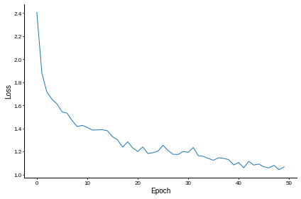
w1_trained, w2_trained = train(ipds_training, spikes_training)Want loss for epoch 1 to be about 2.48, multiply m by constant to get this
Epoch 1: loss=2.40484
Epoch 2: loss=1.87874
Epoch 3: loss=1.71400
Epoch 4: loss=1.65245
Epoch 5: loss=1.61149
Epoch 6: loss=1.54336
Epoch 7: loss=1.53205
Epoch 8: loss=1.46757
Epoch 9: loss=1.41638
Epoch 10: loss=1.42657
Epoch 11: loss=1.40868
Epoch 12: loss=1.38561
Epoch 13: loss=1.38728
Epoch 14: loss=1.38895
Epoch 15: loss=1.37974
Epoch 16: loss=1.32798
Epoch 17: loss=1.30128
Epoch 18: loss=1.23834
Epoch 19: loss=1.28417
Epoch 20: loss=1.23119
Epoch 21: loss=1.19978
Epoch 22: loss=1.23924
Epoch 23: loss=1.18317
Epoch 24: loss=1.18913
Epoch 25: loss=1.20303
Epoch 26: loss=1.25328
Epoch 27: loss=1.20897
Epoch 28: loss=1.17587
Epoch 29: loss=1.17435
Epoch 30: loss=1.20052
Epoch 31: loss=1.19265
Epoch 32: loss=1.23493
Epoch 33: loss=1.16431
Epoch 34: loss=1.15774
Epoch 35: loss=1.13995
Epoch 36: loss=1.12417
Epoch 37: loss=1.14542
Epoch 38: loss=1.14057
Epoch 39: loss=1.13011
Epoch 40: loss=1.08344
Epoch 41: loss=1.10550
Epoch 42: loss=1.05922
Epoch 43: loss=1.11455
Epoch 44: loss=1.08298
Epoch 45: loss=1.09093
Epoch 46: loss=1.06748
Epoch 47: loss=1.05846
Epoch 48: loss=1.08027
Epoch 49: loss=1.04273
Epoch 50: loss=1.06749
# Analyse
print(f"Chance accuracy level: {100 * 1 / NUM_CLASSES:.1f}%")
run_func = lambda x: snn(x, w1_trained, w2_trained)
analyse_accuracy(ipds_training, spikes_training, run_func, 'Train')

ipds_test, spikes_test = random_ipd_input_signal(batch_size*n_testing_batches)
analyse_accuracy(ipds_test, spikes_test, run_func, 'Test')
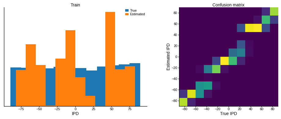
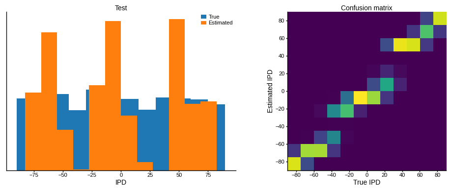
Chance accuracy level: 8.3%
Train classifier accuracy: 59.1%
Train absolute error: 8.0 deg
Test classifier accuracy: 51.2%
Test absolute error: 9.0 deg
def plot_single_weight_mat(ax, w):
    vmax = np.max(np.abs(w))
    im = ax.imshow(w, interpolation='nearest', aspect='auto', origin='lower', vmin=-vmax, vmax=vmax, cmap='seismic')
    ax.set_ylabel('Input neuron index')
    ax.set_xlabel('Hidden layer neuron index')
    ax.figure.colorbar(im, label="Weight", ax=ax)


def plot_weight_mats(w1, w2):
    plt.figure(figsize=(10, 4), dpi=100)
    ax = plt.subplot(121)
    plot_single_weight_mat(ax, w1.detach().cpu().numpy())

    ax = plt.subplot(122)
    plot_single_weight_mat(ax, w2.detach().cpu().numpy())

    plt.tight_layout()


plot_weight_mats(w1_trained, w2_trained)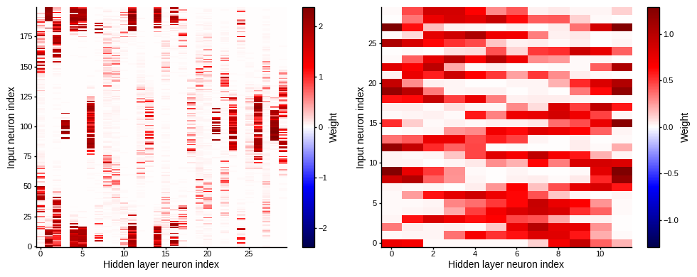
def plot_weight_mats_sorted(w1, w2):
    w1 = w1.detach().cpu().numpy()
    w2 = w2.detach().cpu().numpy()

    # for each column of w1, compute the weighted mean and re-order according to that
    #A = np.arange(w1.shape[0])[:, None]
    A = np.hstack([np.arange(ANF_PER_EAR), -np.arange(ANF_PER_EAR)])[:, None]
    weighted_mean = np.mean((A*w1), axis=0)
    weighted_mean[np.max(w1, axis=0)<.5] = np.inf
    I = np.argsort(weighted_mean)
    w1 = w1[:, I]
    w2 = w2[I, :]

    # Plot the re-ordered weight matrices
    plt.figure(figsize=(10, 3), dpi=100)
    ax = plt.subplot(131)
    plot_single_weight_mat(ax, w1)
    ax.set_ylabel('Input neuron index')
    ax.set_xlabel('Hidden layer neuron index')
    ax.set_title('$W_1$')

    ax = plt.subplot(132)
    plot_single_weight_mat(ax, w2)
    ax.set_ylabel('Hidden layer neuron index')
    ax.set_xlabel('Output neuron index')
    ax.set_title('$W_2$')

    ax = plt.subplot(133)
    plot_single_weight_mat(ax, w1@w2)
    ax.set_ylabel('Input neuron index')
    ax.set_xlabel('Output neuron index')
    ax.set_title('$W_1W_2$')

    plt.tight_layout()

    # Plot some sample weights for hidden neurons

    big_weights = np.max(np.abs(w1), axis=0) > .5

    to_show_count = 15

    best_idcs = np.argsort(big_weights)[::-1][:to_show_count]


    fig, axs = plt.subplots(ncols=5, nrows=to_show_count // 5, dpi=150, sharex='all', sharey='all', constrained_layout=True)

    phi = np.linspace(-np.pi/2, np.pi/2, w1.shape[0]//2)

    for i, j in enumerate(best_idcs):

        ax = axs.ravel()[i]

        ax.plot(phi*180/np.pi, w1[:w1.shape[0]//2, j], label="Left ear")

        ax.plot(phi*180/np.pi, w1[w1.shape[0]//2:, j], label="Right ear")

    plt.suptitle("Individual $W_1$ weights")
    plt.legend(loc='best')
    plt.xlabel('Phase delay (deg)')

plot_weight_mats_sorted(w1_trained, w2_trained)
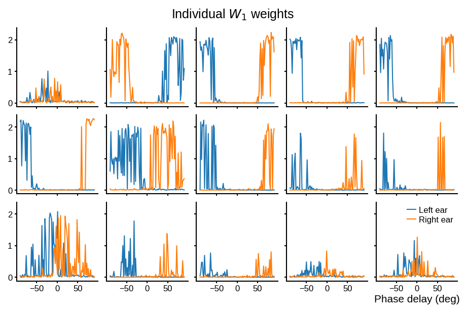
Note a diagonal trend in W1 as well single contiguous bumps in columns of W2, suggesting a preference for coincidence detection. However the accuracy gets much worse (50% on test).
def plot_traces(ax, traces):
    cmap = matplotlib.cm.get_cmap('hsv')
    norm = matplotlib.colors.Normalize(vmin=-180, vmax=+180)

    c = continuise(np.arange(traces.shape[0])) * 180/np.pi
    totals = np.sum(traces, axis=1)
    z_sorting = np.argsort(totals)[::1]


    for j in z_sorting:
        trace = traces[j]
        color = cmap(norm(c[j]))
        ax.plot(trace, color=color)

    sm = matplotlib.cm.ScalarMappable(norm=norm, cmap=cmap)
    sm.set_array(c)
    ax.figure.colorbar(sm, ax=ax, label='ipd')


def plot_single_run(angle, example_input, s_rec, v_rec):
    f, axs = plt.subplots(nrows=4, sharex='all', figsize=(4, 4), dpi=150, constrained_layout=True)

    f.suptitle(f'true angle: {angle*180/np.pi}')

    ax = axs[0]
    ax.imshow(example_input.T, aspect='auto', interpolation='nearest', origin='lower', cmap=plt.cm.gray_r)
    ax.set(
        ylabel='uV',
        title='spikes input neurons',
    )

    ax = axs[1]
    ax.imshow(s_rec.T, aspect='auto', interpolation='nearest', origin='lower', cmap=plt.cm.gray_r)
    ax.set(
        ylabel='uV',
        title='spikes hidden neurons',
    )

    ax = axs[2]
    plot_traces(ax, v_rec.T)
    ax.set(
        ylabel='uV',
        title='mem. output neurons',
    )

    ax = axs[3]
    plot_traces(ax, np.cumsum(v_rec.T, axis=1))
    ax.set(
        xlabel='time',
        ylabel='uV',
        title='cum. mem. output neurons',
    )

def study_single_example(angle, w1, w2):
    example_input = spikes_from_fixed_idp_input_signal(np.array([angle]))

    tau = 2 * MS

    s_rec = layer1(example_input, w1, tau)
    v_rec = layer2(s_rec, w2, tau)

    example_input = example_input[0]
    s_rec = s_rec.detach().numpy()[0]
    v_rec = v_rec.detach().numpy()[0]

    plot_single_run(angle, example_input, s_rec, v_rec)


study_single_example(np.pi * 0.5, w1_trained, w2_trained)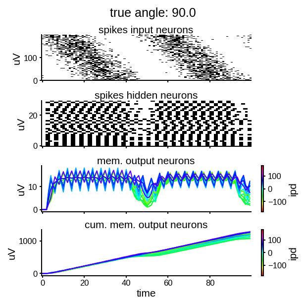
Looking a bit at membrane traces of the output neurions, it seems like the decision is taken mostly in the trough of the sinusoid input, probably because in that period the FRs are low enough that coincidence is more significative for the discrimination.
Further work
Fix gradient of ABS at 0.
Reduce firing rates of AFN. What are realistic values?
Check out Blake Richards’ work showing that you can train ANNs following Dale’s law without loss of performance.