!pip install scikit-learn
!pip install seaborn
!pip install git+https://github.com/neurostatslab/tensortools
Requirement already satisfied: scikit-learn in c:\users\ghosh\anaconda3\envs\spikeloc\lib\site-packages (1.6.1)
Requirement already satisfied: threadpoolctl>=3.1.0 in c:\users\ghosh\anaconda3\envs\spikeloc\lib\site-packages (from scikit-learn) (3.5.0)
Requirement already satisfied: numpy>=1.19.5 in c:\users\ghosh\anaconda3\envs\spikeloc\lib\site-packages (from scikit-learn) (1.23.5)
Requirement already satisfied: joblib>=1.2.0 in c:\users\ghosh\anaconda3\envs\spikeloc\lib\site-packages (from scikit-learn) (1.4.2)
Requirement already satisfied: scipy>=1.6.0 in c:\users\ghosh\anaconda3\envs\spikeloc\lib\site-packages (from scikit-learn) (1.9.3)
Requirement already satisfied: seaborn in c:\users\ghosh\anaconda3\envs\spikeloc\lib\site-packages (0.13.2)
Requirement already satisfied: matplotlib!=3.6.1,>=3.4 in c:\users\ghosh\anaconda3\envs\spikeloc\lib\site-packages (from seaborn) (3.6.2)
Requirement already satisfied: numpy!=1.24.0,>=1.20 in c:\users\ghosh\anaconda3\envs\spikeloc\lib\site-packages (from seaborn) (1.23.5)
Requirement already satisfied: pandas>=1.2 in c:\users\ghosh\anaconda3\envs\spikeloc\lib\site-packages (from seaborn) (2.2.3)
Requirement already satisfied: fonttools>=4.22.0 in c:\users\ghosh\anaconda3\envs\spikeloc\lib\site-packages (from matplotlib!=3.6.1,>=3.4->seaborn) (4.38.0)
Requirement already satisfied: pyparsing>=2.2.1 in c:\users\ghosh\anaconda3\envs\spikeloc\lib\site-packages (from matplotlib!=3.6.1,>=3.4->seaborn) (3.0.9)
Requirement already satisfied: python-dateutil>=2.7 in c:\users\ghosh\anaconda3\envs\spikeloc\lib\site-packages (from matplotlib!=3.6.1,>=3.4->seaborn) (2.8.2)
Requirement already satisfied: pillow>=6.2.0 in c:\users\ghosh\anaconda3\envs\spikeloc\lib\site-packages (from matplotlib!=3.6.1,>=3.4->seaborn) (9.2.0)
Requirement already satisfied: cycler>=0.10 in c:\users\ghosh\anaconda3\envs\spikeloc\lib\site-packages (from matplotlib!=3.6.1,>=3.4->seaborn) (0.11.0)
Requirement already satisfied: contourpy>=1.0.1 in c:\users\ghosh\anaconda3\envs\spikeloc\lib\site-packages (from matplotlib!=3.6.1,>=3.4->seaborn) (1.0.6)
Requirement already satisfied: packaging>=20.0 in c:\users\ghosh\anaconda3\envs\spikeloc\lib\site-packages (from matplotlib!=3.6.1,>=3.4->seaborn) (21.3)
Requirement already satisfied: kiwisolver>=1.0.1 in c:\users\ghosh\anaconda3\envs\spikeloc\lib\site-packages (from matplotlib!=3.6.1,>=3.4->seaborn) (1.4.4)
Requirement already satisfied: tzdata>=2022.7 in c:\users\ghosh\anaconda3\envs\spikeloc\lib\site-packages (from pandas>=1.2->seaborn) (2024.2)
Requirement already satisfied: pytz>=2020.1 in c:\users\ghosh\anaconda3\envs\spikeloc\lib\site-packages (from pandas>=1.2->seaborn) (2022.6)
Requirement already satisfied: six>=1.5 in c:\users\ghosh\anaconda3\envs\spikeloc\lib\site-packages (from python-dateutil>=2.7->matplotlib!=3.6.1,>=3.4->seaborn) (1.16.0)
Collecting git+https://github.com/neurostatslab/tensortools
Cloning https://github.com/neurostatslab/tensortools to c:\users\ghosh\appdata\local\temp\pip-req-build-tofimbdt
Resolved https://github.com/neurostatslab/tensortools to commit 9e732ac5f27e8f993751122ad0d09f1318528bf5
Preparing metadata (setup.py): started
Preparing metadata (setup.py): finished with status 'done'
Requirement already satisfied: numpy in c:\users\ghosh\anaconda3\envs\spikeloc\lib\site-packages (from tensortools==0.4) (1.23.5)
Requirement already satisfied: scipy in c:\users\ghosh\anaconda3\envs\spikeloc\lib\site-packages (from tensortools==0.4) (1.9.3)
Requirement already satisfied: tqdm in c:\users\ghosh\anaconda3\envs\spikeloc\lib\site-packages (from tensortools==0.4) (4.64.1)
Requirement already satisfied: munkres in c:\users\ghosh\anaconda3\envs\spikeloc\lib\site-packages (from tensortools==0.4) (1.1.4)
Requirement already satisfied: numba in c:\users\ghosh\anaconda3\envs\spikeloc\lib\site-packages (from tensortools==0.4) (0.56.4)
Requirement already satisfied: matplotlib in c:\users\ghosh\anaconda3\envs\spikeloc\lib\site-packages (from tensortools==0.4) (3.6.2)
Requirement already satisfied: kiwisolver>=1.0.1 in c:\users\ghosh\anaconda3\envs\spikeloc\lib\site-packages (from matplotlib->tensortools==0.4) (1.4.4)
Requirement already satisfied: pillow>=6.2.0 in c:\users\ghosh\anaconda3\envs\spikeloc\lib\site-packages (from matplotlib->tensortools==0.4) (9.2.0)
Requirement already satisfied: pyparsing>=2.2.1 in c:\users\ghosh\anaconda3\envs\spikeloc\lib\site-packages (from matplotlib->tensortools==0.4) (3.0.9)
Requirement already satisfied: cycler>=0.10 in c:\users\ghosh\anaconda3\envs\spikeloc\lib\site-packages (from matplotlib->tensortools==0.4) (0.11.0)
Requirement already satisfied: fonttools>=4.22.0 in c:\users\ghosh\anaconda3\envs\spikeloc\lib\site-packages (from matplotlib->tensortools==0.4) (4.38.0)
Requirement already satisfied: contourpy>=1.0.1 in c:\users\ghosh\anaconda3\envs\spikeloc\lib\site-packages (from matplotlib->tensortools==0.4) (1.0.6)
Requirement already satisfied: packaging>=20.0 in c:\users\ghosh\anaconda3\envs\spikeloc\lib\site-packages (from matplotlib->tensortools==0.4) (21.3)
Requirement already satisfied: python-dateutil>=2.7 in c:\users\ghosh\anaconda3\envs\spikeloc\lib\site-packages (from matplotlib->tensortools==0.4) (2.8.2)
Requirement already satisfied: setuptools in c:\users\ghosh\anaconda3\envs\spikeloc\lib\site-packages (from numba->tensortools==0.4) (65.5.1)
Requirement already satisfied: llvmlite<0.40,>=0.39.0dev0 in c:\users\ghosh\anaconda3\envs\spikeloc\lib\site-packages (from numba->tensortools==0.4) (0.39.1)
Requirement already satisfied: colorama in c:\users\ghosh\anaconda3\envs\spikeloc\lib\site-packages (from tqdm->tensortools==0.4) (0.4.6)
Requirement already satisfied: six>=1.5 in c:\users\ghosh\anaconda3\envs\spikeloc\lib\site-packages (from python-dateutil>=2.7->matplotlib->tensortools==0.4) (1.16.0)
Running command git clone --filter=blob:none --quiet https://github.com/neurostatslab/tensortools 'C:\Users\ghosh\AppData\Local\Temp\pip-req-build-tofimbdt'
TCA Analysis
Duplicate this notebook and experiment away.
See How to Contribute (steps 4 and 5) for help with this.
In this notebook (which is based on the third notebook of the 2022 Cosyne tutorial), we’re going to use surrogate gradient descent to find a solution to the sound localisation problem. The surrogate gradient descent approach and code is heavily inspired by (certainly not stolen) from Friedemann Zenke’s SPyTorch tutorial, which I recommend for a deeper dive into the maths.
import os

import numpy as np
import matplotlib.pyplot as plt
from matplotlib.gridspec import GridSpec
from sklearn.decomposition import PCA
from sklearn.manifold import TSNE

import torch
import torch.nn as nn

dtype = torch.float

# Check whether a GPU is available
# if torch.backends.mps.is_available():
#     device = torch.device("mps")  # Use Apple's Metal Performance Shaders
# el
if torch.cuda.is_available():
    device = torch.device("cuda")
else:
    device = torch.device("cpu")

print(f"Using device: {device}")
my_computer_is_slow = True  # set this to True if using Colab

fig_counter = 0
Using device: cpu
Sound localization stimuli
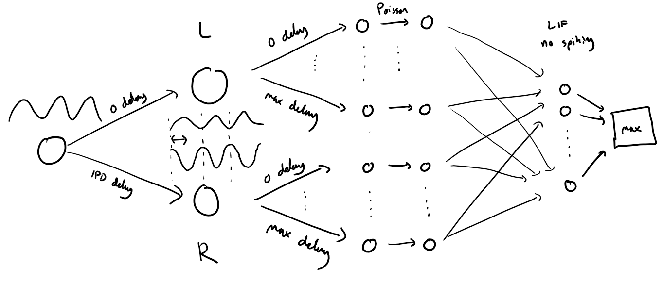
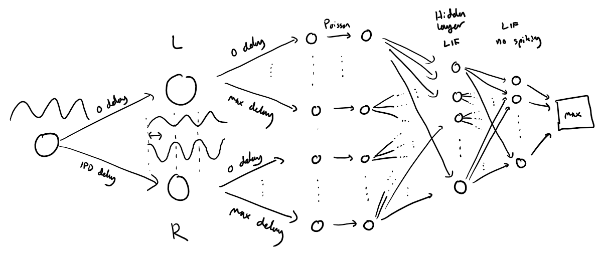
The following function creates a set of stimuli that can be used for training or testing. We have two ears (0 and 1), and ear 1 will get a version of the signal delayed by an IPD we can write as in equations (ipd in code). The basic signal is a sine wave as in the previous notebook, made positive, so . In addition, for each ear there will be neurons per ear (anf_per_ear because these are auditory nerve fibres). Each neuron generates Poisson spikes at a certain firing rate, and these Poisson spike trains are independent. In addition, since it is hard to train delays, we seed it with uniformly distributed delays from a minimum of 0 to a maximum of in each ear, so that the differences between the two ears can cover the range of possible IPDs ( to ). We do this directly by adding a phase delay to each neuron. So for ear and neuron at time the angle . Finally, we generate Poisson spike trains with a rate . (rate_max) is the maximum instantaneous firing rate, and (envelope_power) is a constant that sharpens the envelope. The higher and the easier the problem (try it out on the cell below to see why).
Here’s a picture of the architecture for the stimuli:

The functions below return two arrays ipd and spikes. ipd is an array of length num_samples that gives the true IPD, and spikes is an array of 0 (no spike) and 1 (spike) of shape (num_samples, duration_steps, 2*anf_per_ear), where duration_steps is the number of time steps there are in the stimulus.
# Not using Brian so we just use these constants to make equations look nicer below
second = 1
ms = 1e-3
Hz = 1

# Stimulus and simulation parameters
dt = 1 * ms  # large time step to make simulations run faster for tutorial
anf_per_ear = 100  # repeats of each ear with independent noise
envelope_power = 2  # higher values make sharper envelopes, easier
rate_max = 600 * Hz  # maximum Poisson firing rate
f = 20 * Hz  # stimulus frequency
duration = 0.1 * second  # stimulus duration
# duration = duration / 2
duration_steps = int(np.round(duration / dt))
input_size = 2 * anf_per_ear

# Generate an input signal (spike array) from array of true IPDs
def input_signal(ipd):
    num_samples = len(ipd)
    T = np.arange(duration_steps) * dt  # array of times
    phi = (
        2 * np.pi * (f * T + np.random.rand())
    )  # array of phases corresponding to those times with random offset
    # each point in the array will have a different phase based on which ear it is
    # and its delay
    theta = np.zeros((num_samples, duration_steps, 2 * anf_per_ear))
    # for each ear, we have anf_per_ear different phase delays from to pi/2 so
    # that the differences between the two ears can cover the full range from -pi/2 to pi/2
    phase_delays = np.linspace(0, np.pi / 2, anf_per_ear)
    # now we set up these theta to implement that. Some numpy vectorisation logic here which looks a little weird,
    # but implements the idea in the text above.
    theta[:, :, :anf_per_ear] = (
        phi[np.newaxis, :, np.newaxis] + phase_delays[np.newaxis, np.newaxis, :]
    )
    theta[:, :, anf_per_ear:] = (
        phi[np.newaxis, :, np.newaxis]
        + phase_delays[np.newaxis, np.newaxis, :]
        + ipd[:, np.newaxis, np.newaxis]
    )
    # now generate Poisson spikes at the given firing rate as in the previous notebook
    spikes = (
        np.random.rand(num_samples, duration_steps, 2 * anf_per_ear)
        < rate_max * dt * (0.5 * (1 + np.sin(theta))) ** envelope_power
    )
    return spikes


# Generate some true IPDs from U(-pi/2, pi/2) and corresponding spike arrays
def random_ipd_input_signal(num_samples, tensor=True):
    ipd = (
        np.random.rand(num_samples) * np.pi - np.pi / 2
    )  # uniformly random in (-pi/2, pi/2)
    spikes = input_signal(ipd)
    if tensor:
        ipd = torch.tensor(ipd, device=device, dtype=dtype)
        spikes = torch.tensor(spikes, device=device, dtype=dtype)
    return ipd, spikes


def random_step_ipd_input_signal(num_samples, tensor=True):
    # Generate IPDs linearly spaced from -pi/2 to pi/2
    ipd = np.linspace(-np.pi / 2, np.pi / 2, num_samples)
    # Generate the corresponding spike arrays
    spikes = input_signal(ipd)
    if tensor:
        ipd = torch.tensor(ipd, device=device, dtype=dtype)
        spikes = torch.tensor(spikes, device=device, dtype=dtype)
    return ipd, spikes


# Plot a few just to show how it looks
ipd, spikes = random_ipd_input_signal(8)
spikes = spikes.cpu()
plt.figure(figsize=(10, 4), dpi=100)
for i in range(8):
    plt.subplot(2, 4, i + 1)
    plt.imshow(
        spikes[i, :, :].T, aspect="auto", interpolation="nearest", cmap=plt.cm.gray_r
    )
    plt.title(f"True IPD = {int(ipd[i]*180/np.pi)} deg")
    if i >= 4:
        plt.xlabel("Time (steps)")
    if i % 4 == 0:
        plt.ylabel("Input neuron index")
plt.tight_layout()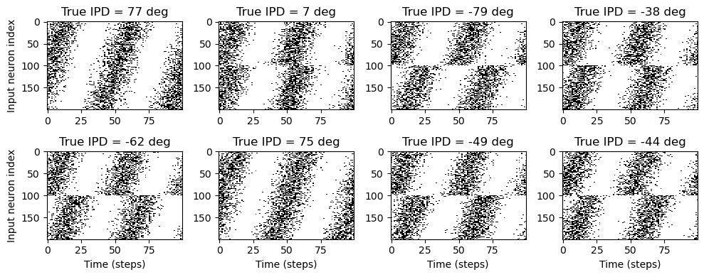
ipd, spikes = random_step_ipd_input_signal(8)
spikes = spikes.cpu()
plt.figure(figsize=(10, 4), dpi=100)
for i in range(8):
    plt.subplot(2, 4, i + 1)
    plt.imshow(
        spikes[i, :, :].T, aspect="auto", interpolation="nearest", cmap=plt.cm.gray_r
    )
    plt.title(f"True IPD = {int(ipd[i]*180/np.pi)} deg")
    if i >= 4:
        plt.xlabel("Time (steps)")
    if i % 4 == 0:
        plt.ylabel("Input neuron index")
plt.tight_layout()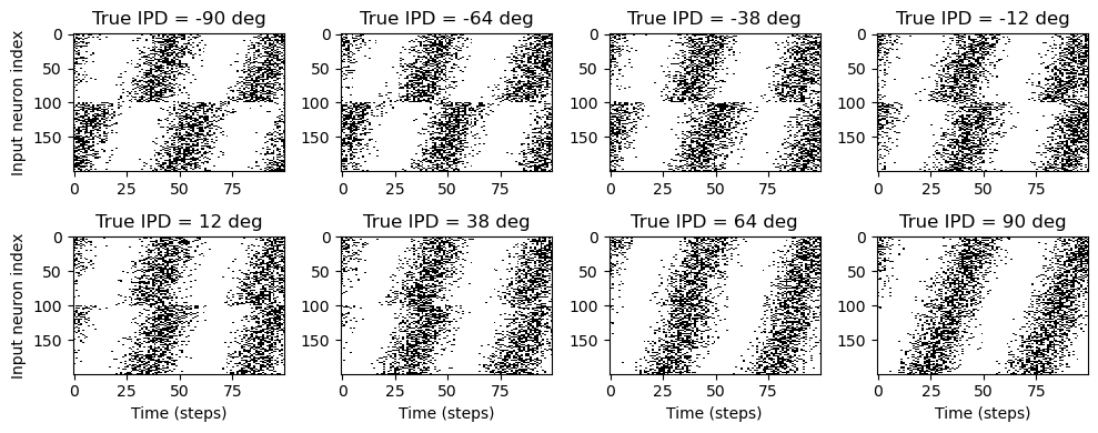
Now the aim is to take these input spikes and infer the IPD. We can do this either by discretising and using a classification approach, or with a regression approach. For the moment, let’s try it with a classification approach.
Training
We train this by dividing the input data into batches and computing gradients across batches. In this notebook, batch and data size is small so that it can be run on a laptop in a couple of minutes, but normally you’d use larger batches and more data. Let’s start with the data.
# Parameters for training. These aren't optimal, but instead designed
# to give a reasonable result in a small amount of time for the tutorial!
if my_computer_is_slow:
    batch_size = 64
    n_training_batches = 64
else:
    batch_size = 128
    n_training_batches = 128
n_testing_batches = 32
num_samples = batch_size * n_training_batches


# Generator function iterates over the data in batches
# We randomly permute the order of the data to improve learning
def data_generator(ipds, spikes, random=True):
    if random:
        perm = torch.randperm(spikes.shape[0])
        spikes = spikes[perm, :, :]
        ipds = ipds[perm]
    n, _, _ = spikes.shape
    n_batch = n // batch_size
    for i in range(n_batch):
        x_local = spikes[i * batch_size : (i + 1) * batch_size, :, :]
        y_local = ipds[i * batch_size : (i + 1) * batch_size]
        yield x_local, y_local
Classification approach
We discretise the IPD range of into (num_classes) equal width segments. Replace angle with the integer part (floor) of . We also convert the arrays into PyTorch tensors for later use. The algorithm will now guess the index of the segment, converting that to the midpoint of the segment when needed.
The algorithm will work by outputting a length vector and the index of the maximum value of y will be the guess as to the class (1-hot encoding), i.e. . We will perform the training with a softmax and negative loss likelihood loss, which is a standard approach in machine learning.
# classes at 15 degree increments
num_classes = 180 // 15
print(f"Number of classes = {num_classes}")


def discretise(ipds):
    return ((ipds + np.pi / 2) * num_classes / np.pi).long()  # assumes input is tensor


def continuise(ipd_indices):  # convert indices back to IPD midpoints
    return (ipd_indices + 0.5) / num_classes * np.pi - np.pi / 2
Number of classes = 12
Membrane only (no spiking neurons)
Before we get to spiking, we’re going to warm up with a non-spiking network that shows some of the features of the full model but without any coincidence detection, it can’t do the task. We basically create a neuron model that has everything except spiking, so the membrane potential dynamics are there and it takes spikes as input. The neuron model we’ll use is just the LIF model we’ve already seen. We’ll use a time constant of 20 ms, and we pre-calculate a constant so that updating the membrane potential is just multiplying by (as we saw in the first notebook). We store the input spikes in a vector of 0s and 1s for each time step, and multiply by the weight matrix to get the input, i.e. .
We initialise the weight matrix uniformly with bounds proportionate to the inverse square root of the number of inputs (fairly standard, and works here).
The output of this will be a vector of (num_classes) membrane potential traces. We sum these traces over time and use this as the output vector (the largest one will be our prediction of the class and therefore the IPD).
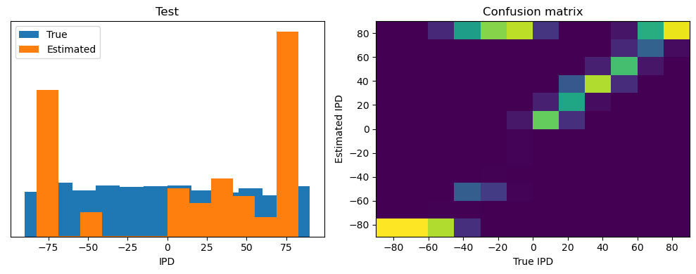
Analysis of results
Now we compute the training and test accuracy, and plot histograms and confusion matrices to understand the errors it’s making.
This function evaluates the performance of a classifier on given data.
Parameters: ipds (numpy.ndarray): Inter-pulse intervals data. spikes (numpy.ndarray): Spike train data. label (str): Label to be used for the output (e.g., ‘Train’ or ‘Test’). run (function): Classifier function to be evaluated.
The function works by iterating over the data generated by the data_generator function. For each batch of data:
It gets the true labels and discretizes them.
It runs the classifier on the input data.
It sums the classifier’s output over the time dimension and finds the class with the highest output.
It calculates the accuracy of the classifier by comparing the predicted classes to the true labels.
It updates the confusion matrix based on the true and predicted classes.
It stores the true and estimated labels, and the accuracy for this batch.
After going through all the data, it calculates the overall accuracy and absolute error, and prints them. It also plots two histograms: one for the true labels and one for the estimated labels, and a normalized confusion matrix.
def analyse(ipds, spikes, label, run):
    accs = []
    ipd_true = []
    ipd_est = []
    confusion = np.zeros((num_classes, num_classes))
    for x_local, y_local in data_generator(ipds, spikes):
        y_local_orig = y_local
        y_local = discretise(y_local)
        output = run(x_local)
        m = torch.sum(output, 1)  # Sum time dimension
        _, am = torch.max(m, 1)  # argmax over output units
        tmp = np.mean((y_local == am).detach().cpu().numpy())  # compare to labels
        for i, j in zip(y_local.detach().cpu().numpy(), am.detach().cpu().numpy()):
            confusion[j, i] += 1
        ipd_true.append(y_local_orig.detach().cpu().numpy())
        ipd_est.append(continuise(am.detach().cpu().numpy()))
        accs.append(tmp)
    ipd_true = np.hstack(ipd_true)
    ipd_est = np.hstack(ipd_est)
    abs_errors_deg = abs(ipd_true - ipd_est) * 180 / np.pi
    print()
    print(f"{label} classifier accuracy: {100*np.mean(accs):.1f}%")
    print(f"{label} absolute error: {np.mean(abs_errors_deg):.1f} deg")

    plt.figure(figsize=(10, 4), dpi=100)
    plt.subplot(121)
    plt.hist(ipd_true * 180 / np.pi, bins=num_classes, label="True")
    plt.hist(ipd_est * 180 / np.pi, bins=num_classes, label="Estimated")
    plt.xlabel("IPD")
    plt.yticks([])
    plt.legend(loc="best")
    plt.title(label)
    plt.subplot(122)
    confusion /= np.sum(confusion, axis=0)[np.newaxis, :]
    plt.imshow(
        confusion,
        interpolation="nearest",
        aspect="auto",
        origin="lower",
        extent=(-90, 90, -90, 90),
    )
    plt.xlabel("True IPD")
    plt.ylabel("Estimated IPD")
    plt.title("Confusion matrix")
    plt.tight_layout()

    return 100 * np.mean(accs)


# print(f"Chance accuracy level: {100*1/num_classes:.1f}%")
# run_func = lambda x: membrane_only(x, W)
# analyse(ipds, spikes, 'Train', run=run_func)
# ipds_test, spikes_test = random_ipd_input_signal(batch_size*n_testing_batches)
# analyse(ipds_test, spikes_test, 'Test', run=run_func)
This poor performance isn’t surprising because this network is not actually doing any coincidence detection, just a weighted sum of input spikes.
Spiking model
Next we’ll implement a version of the model with spikes to see how that changes performance. We’ll just add a single hidden feed-forward layer of spiking neurons between the input and the output layers. This layer will be spiking, so we need to use the surrogate gradient descent approach.
Surrogate gradient descent
First, this is the key part of surrogate gradient descent, a function where we override the computation of the gradient to replace it with a smoothed gradient. You can see that in the forward pass (method forward) it returns the Heaviside function of the input (takes value 1 if the input is >0) or value 0 otherwise. In the backwards pass, it returns the gradient of a sigmoid function.
beta = 5


class SurrGradSpike(torch.autograd.Function):
    @staticmethod
    def forward(ctx, input):
        ctx.save_for_backward(input)
        out = torch.zeros_like(input)
        out[input > 0] = 1.0
        return out

    @staticmethod
    def backward(ctx, grad_output):
        (input,) = ctx.saved_tensors
        # Original SPyTorch/SuperSpike gradient
        # This seems to be a typo or error? But it works well
        # grad = grad_output/(100*torch.abs(input)+1.0)**2
        # Sigmoid
        grad = (
            grad_output
            * beta
            * torch.sigmoid(beta * input)
            * (1 - torch.sigmoid(beta * input))
        )
        return grad


spike_fn = SurrGradSpike.apply
Updated model
The code for the updated model is very similar to the membrane only layer. First, for initialisation we now need two weight matrices, from the input to the hidden layer, and from the hidden layer to the output layer. Second, we run two passes of the loop that you saw above for the membrane only model.
The first pass computes the output spikes of the hidden layer. The second pass computes the output layer and is exactly the same as before except using the spikes from the hidden layer instead of the input layer.
For the first pass, we modify the function in two ways.
Firstly, we compute the spikes with the line s = spike_fn(v-1). In the forward pass this just computes the Heaviside function of , i.e. returns 1 if , otherwise 0, which is the spike threshold function for the LIF neuron. In the backwards pass, it returns a gradient of the smoothed version of the Heaviside function.
The other line we change is the membrane potential update line. Now, we multiply by where ( if there was a spike in the previous time step, otherwise ), so that the membrane potential is reset to 0 after a spike (but in a differentiable way rather than just setting it to 0).
num_hidden = 30


# Weights and uniform weight initialisation
def init_weight_matrices():
    # Input to hidden layer
    W1 = nn.Parameter(
        torch.empty(
            (input_size, num_hidden), device=device, dtype=dtype, requires_grad=True
        )
    )
    fan_in, _ = nn.init._calculate_fan_in_and_fan_out(W1)
    bound = 1 / np.sqrt(fan_in)
    nn.init.uniform_(W1, -bound, bound)
    # Hidden layer to output
    W2 = nn.Parameter(
        torch.empty(
            (num_hidden, num_classes), device=device, dtype=dtype, requires_grad=True
        )
    )
    fan_in, _ = nn.init._calculate_fan_in_and_fan_out(W2)
    bound = 1 / np.sqrt(fan_in)
    nn.init.uniform_(W2, -bound, bound)
    return W1, W2


# Run the simulation
def snn(input_spikes, W1, W2, tau=20 * ms):
    # First layer: input to hidden
    v = torch.zeros((batch_size, num_hidden), device=device, dtype=dtype)
    s = torch.zeros((batch_size, num_hidden), device=device, dtype=dtype)
    s_rec = [s]
    h = torch.einsum("abc,cd->abd", (input_spikes, W1))
    alpha = np.exp(-dt / tau)
    for t in range(duration_steps - 1):
        new_v = (alpha * v + h[:, t, :]) * (1 - s)  # multiply by 0 after a spike
        s = spike_fn(v - 1)  # threshold of 1
        v = new_v
        s_rec.append(s)
    s_rec = torch.stack(s_rec, dim=1)
    # Second layer: hidden to output
    v = torch.zeros((batch_size, num_classes), device=device, dtype=dtype)
    s = torch.zeros((batch_size, num_classes), device=device, dtype=dtype)
    v_rec = [v]
    h = torch.einsum("abc,cd->abd", (s_rec, W2))
    alpha = np.exp(-dt / tau)
    for t in range(duration_steps - 1):
        v = alpha * v + h[:, t, :]
        v_rec.append(v)
    v_rec = torch.stack(v_rec, dim=1)
    # Return recorded spike trains and membrane potentials
    return s_rec, v_rec
Training and analysing
We train it as before, except that we modify the functions to take the two weight matrices into account.
# Training function with spike recording, including network output IPDs
def train_network(ipds, spikes, nb_epochs, lr, num_classes):
    W1, W2 = init_weight_matrices()
    optimizer = torch.optim.Adam([W1, W2], lr=lr)
    loss_fn = nn.NLLLoss()
    log_softmax_fn = nn.LogSoftmax(dim=1)
    spike_data = []
    input_ipd_data = []
    estimated_ipd_data = []
    loss_hist = []

    for e in range(nb_epochs):
        local_loss = []
        for x_local, y_local in data_generator(discretise(ipds), spikes):
            # Run network
            output = snn(x_local, W1, W2)
            v_rec = output[-1]
            s_rec = output[0]

            # Record spikes and corresponding IPD values
            spike_data.append(s_rec.detach().cpu().numpy())  # Detach and move to CPU
            input_ipd_data.append(y_local.detach().cpu().numpy())

            # Compute cross entropy loss
            m = torch.mean(v_rec, 1)  # Mean across time dimension
            loss = loss_fn(log_softmax_fn(m), y_local)
            local_loss.append(loss.item())

            # Record estimated IPDs
            _, estimated_ipds = torch.max(log_softmax_fn(m), 1)
            estimated_ipd_data.append(estimated_ipds.detach().cpu().numpy())

            # Update gradients
            optimizer.zero_grad()
            loss.backward()
            optimizer.step()

        loss_hist.append(np.mean(local_loss))
        print("Epoch %i: loss=%.5f" % (e + 1, np.mean(local_loss)))

    # Convert lists of data to tensors
    spike_tensor = torch.tensor(np.array(spike_data)).float()
    input_ipd_tensor = torch.tensor(np.array(input_ipd_data)).float()
    estimated_ipd_tensor = torch.tensor(np.array(estimated_ipd_data)).float()

    return W1, W2, spike_tensor, input_ipd_tensor, estimated_ipd_tensor


# Training parameters
nb_epochs = 10  # quick, it won't have converged
lr = 0.01

# Generate the training data
ipds, spikes = random_ipd_input_signal(num_samples)
W1, W2, recorded_spikes, recorded_input_ipds, recorded_estimated_ipds = train_network(
    ipds, spikes, nb_epochs, lr, num_classes
)

print("Recorded spikes shape: ", recorded_spikes.shape)
print("Recorded input IPDs shape: ", recorded_input_ipds.shape)
print("Recorded estimated IPDs shape: ", recorded_estimated_ipds.shape)
# Analyse
print(f"Chance accuracy level: {100*1/num_classes:.1f}%")
run_func = lambda x: snn(x, W1, W2)[-1]
analyse(ipds, spikes, "Train", run=run_func)
ipds_test, spikes_test = random_ipd_input_signal(batch_size * n_testing_batches)
analyse(ipds_test, spikes_test, "Test", run=run_func)
Epoch 1: loss=2.04972
Epoch 2: loss=1.26993
Epoch 3: loss=0.92173
Epoch 4: loss=0.77729
Epoch 5: loss=0.70641
Epoch 6: loss=0.63097
Epoch 7: loss=0.58728
Epoch 8: loss=0.58160
Epoch 9: loss=0.55290
Epoch 10: loss=0.50821
Recorded spikes shape: torch.Size([640, 64, 100, 30])
Recorded input IPDs shape: torch.Size([640, 64])
Recorded estimated IPDs shape: torch.Size([640, 64])
Chance accuracy level: 8.3%
Train classifier accuracy: 83.1%
Train absolute error: 4.7 deg
Test classifier accuracy: 42.6%
Test absolute error: 30.6 deg
42.578125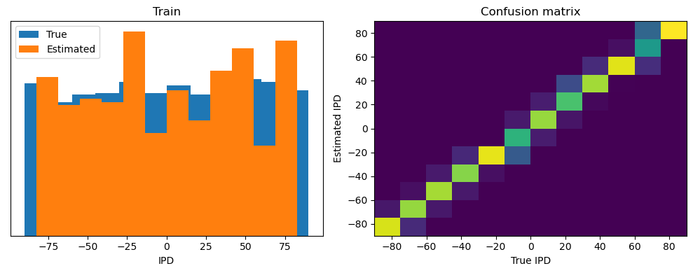
TCA
from tensortools.cpwarp import ShiftedCP, fit_shifted_cp
import tensortools as tt
from scipy.ndimage import gaussian_filter1d

n_trials = 100  # 1
N_RESTARTS = 5
MAX_SHIFT = 0.15
def plot_result_with_ipd_coloring(
m, ipds, titles=("Trial", "Neuron", "Time"), vertical_layout=True
):
num_ranks = len(m.factors[0])
colors = plt.cm.get_cmap("tab20", num_ranks)
if vertical_layout:
n_rows = num_ranks
n_cols = len(m.factors)
else:
n_rows = len(m.factors)
n_cols = num_ranks
# Create subplots
fig, axes = plt.subplots(n_rows, n_cols, figsize=(3 * n_cols, 2 * n_rows))
if n_rows * n_cols == 1:
axes = np.array([[axes]]) # Double bracket to make it 2D
elif n_rows == 1 or n_cols == 1:
axes = axes.reshape(n_rows, n_cols) # Ensure axes is always a 2D array
def normalize(f):
return f / np.linalg.norm(f)
# Plot each factor in each mode
for i in range(n_rows):
for j in range(n_cols):
ax = axes[i, j]
factor = m.factors[j][i] if vertical_layout else m.factors[i][j]
norm_factor = normalize(factor)
if j == 0: # Trial factors
# Scatter plot for trial factors
scatter = ax.scatter(
range(len(norm_factor)),
norm_factor,
c=continuise(ipds),
cmap="viridis",
edgecolor="k",
)
fig.colorbar(scatter, ax=ax, label="IPD")
ax.set_title(f"{titles[j]} Factor {i+1}")
elif j == 1: # Neuron factors
# Bar plot for neuron factors
ax.bar(range(len(norm_factor)), norm_factor, color="blue")
ax.set_title(f"{titles[j]} Factor {i+1}")
else: # Time factors
# Line plot for time factors
ax.plot(norm_factor, color=colors(i))
ax.set_title(f"{titles[j]} Factor {i+1}")
ax.spines["top"].set_visible(False)
ax.spines["right"].set_visible(False)
if i == n_rows - 1:
ax.set_xlabel(titles[j], labelpad=0)
if j == 0:
ax.set_ylabel("Activation")
plt.tight_layout()
return figDuring training analysis:
This tensor represents the recorded spikes across 640 iterations (10 epochs × 64 batches per epoch). 640: Represents each batch processed across all epochs. 64: Each entry within the batch represents one sample, and there are 64 samples per batch. 100: Represents the duration steps, i.e., the number of time steps for which the neural activity is recorded (100 ms in your setup). 30: Represents the number of neurons in the hidden layer for which you’re recording spikes.
def transform_spikes(recorded_spikes, sigma=2.0):
    # convert to NumPy array
    if isinstance(recorded_spikes, torch.Tensor):
        recorded_spikes = recorded_spikes.cpu().numpy().astype(np.float64)

    # collapse the first two dimensions (epochs*batches and batch_size)
    reshaped_spikes = recorded_spikes.reshape(
        -1, recorded_spikes.shape[2], recorded_spikes.shape[3]
    )

    # Change from [total_samples, time, neurons] to [total_samples, neurons, time]
    reshaped_spikes = np.transpose(reshaped_spikes, (0, 2, 1))

    # Apply Gaussian smoothing along the time axis for each neuron
    smoothed_spikes = np.zeros_like(reshaped_spikes)
    for i in range(reshaped_spikes.shape[0]):
        for j in range(reshaped_spikes.shape[1]):
            smoothed_spikes[i, j, :] = gaussian_filter1d(
                reshaped_spikes[i, j, :], sigma=sigma
            )

    return smoothed_spikes


# Convert the recorded spikes into a reshaped tensor
spikes_tensor = transform_spikes(recorded_spikes)
print("Shape of spikes_tensor:", spikes_tensor.shape)
# This will reshape [640, 64] to [40960]
recorded_input_ipds = recorded_input_ipds.view(-1)
recorded_ipds = recorded_input_ipds.detach().cpu().numpy().astype(np.float64)
recorded_estimated_ipds = (
    recorded_estimated_ipds.view(-1).detach().cpu().numpy().astype(np.float64)
)
recorded_ipds.flatten()
recorded_estimated_ipds.flatten()
print("Shape of recorded_ipds:", recorded_input_ipds.shape)
print("Shape of recorded_estimated_ipds:", recorded_estimated_ipds.shape)
Shape of spikes_tensor: (40960, 30, 100)
Shape of recorded_ipds: torch.Size([40960])
Shape of recorded_estimated_ipds: (40960,)
# Define the sampling rate
divide_by = 500

# Sample every 'divide_by' sample across all tensors
spikes_tensor = spikes_tensor[::divide_by]
recorded_ipds = recorded_ipds[::divide_by]
recorded_estimated_ipds = recorded_estimated_ipds[::divide_by]

# Print the shapes to confirm the operation
print("Shape of spikes_tensor:", spikes_tensor.shape)
print("Shape of recorded_ipds:", recorded_ipds.shape)
print("Shape of recorded_estimated_ipds:", recorded_estimated_ipds.shape)
Shape of spikes_tensor: (82, 30, 100)
Shape of recorded_ipds: (82,)
Shape of recorded_estimated_ipds: (82,)
# Optimum num of components using reconstruction error
num_components = 15
# Fit an ensemble of models, 4 random replicates / optimization runs per model rank
ensemble = tt.Ensemble(fit_method="ncp_hals")
ensemble.fit(spikes_tensor, ranks=range(1, num_components), replicates=5) # range(1,32)
fig, axes = plt.subplots(1, 2)
# plot reconstruction error as a function of num components.
tt.plot_objective(ensemble, ax=axes[0])
# plot model similarity as a function of num components.
tt.plot_similarity(ensemble, ax=axes[1])
fig.tight_layout()
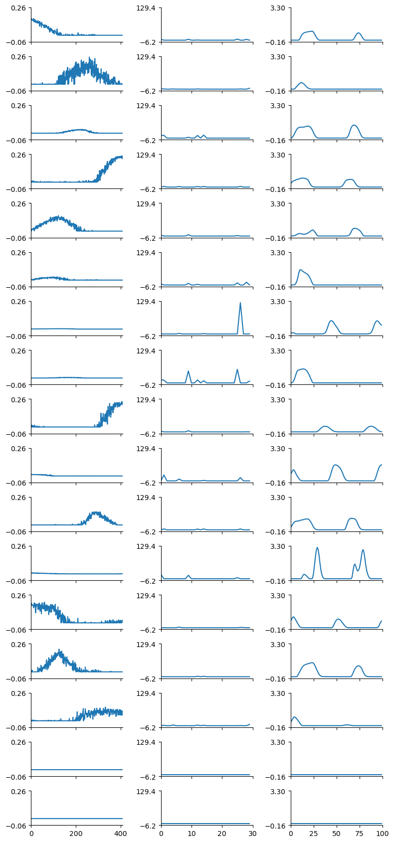
# Plot the low-d factors
replicate = 0
tt.plot_factors(ensemble.factors(num_components - 1)[replicate])
# plt.show()Fitting rank-1 models: 0%| | 0/5 [00:00<?, ?it/s]c:\Users\ghosh\anaconda3\envs\spikeloc\lib\site-packages\tensortools\optimize\ncp_hals.py:185: NumbaPerformanceWarning: '@' is faster on contiguous arrays, called on (array(float64, 2d, C), array(float64, 1d, A))
Cp = factors[:, idx] @ grams[idx][:, p]
c:\Users\ghosh\anaconda3\envs\spikeloc\lib\site-packages\numba\core\typing\npydecl.py:913: NumbaPerformanceWarning: '@' is faster on contiguous arrays, called on (array(float64, 2d, C), array(float64, 1d, A))
warnings.warn(NumbaPerformanceWarning(msg))
Rank-1 models: min obj, 0.77; max obj, 0.77; time to fit, 2.5s
Rank-2 models: min obj, 0.61; max obj, 0.61; time to fit, 0.2s
Rank-3 models: min obj, 0.55; max obj, 0.58; time to fit, 0.3s
Rank-4 models: min obj, 0.50; max obj, 0.53; time to fit, 0.3s
Rank-5 models: min obj, 0.47; max obj, 0.51; time to fit, 0.3s
Rank-6 models: min obj, 0.44; max obj, 0.51; time to fit, 0.5s
Rank-7 models: min obj, 0.42; max obj, 0.45; time to fit, 0.6s
Rank-8 models: min obj, 0.41; max obj, 0.43; time to fit, 0.6s
Rank-9 models: min obj, 0.39; max obj, 0.40; time to fit, 0.9s
Rank-10 models: min obj, 0.38; max obj, 0.41; time to fit, 0.7s
Rank-11 models: min obj, 0.37; max obj, 0.39; time to fit, 1.3s
Rank-12 models: min obj, 0.36; max obj, 0.40; time to fit, 1.3s
Rank-13 models: min obj, 0.35; max obj, 0.38; time to fit, 1.3s
Rank-14 models: min obj, 0.35; max obj, 0.36; time to fit, 0.6s
(<Figure size 800x1400 with 42 Axes>,
 array([[<AxesSubplot: >, <AxesSubplot: >, <AxesSubplot: >],
        [<AxesSubplot: >, <AxesSubplot: >, <AxesSubplot: >],
        [<AxesSubplot: >, <AxesSubplot: >, <AxesSubplot: >],
        [<AxesSubplot: >, <AxesSubplot: >, <AxesSubplot: >],
        [<AxesSubplot: >, <AxesSubplot: >, <AxesSubplot: >],
        [<AxesSubplot: >, <AxesSubplot: >, <AxesSubplot: >],
        [<AxesSubplot: >, <AxesSubplot: >, <AxesSubplot: >],
        [<AxesSubplot: >, <AxesSubplot: >, <AxesSubplot: >],
        [<AxesSubplot: >, <AxesSubplot: >, <AxesSubplot: >],
        [<AxesSubplot: >, <AxesSubplot: >, <AxesSubplot: >],
        [<AxesSubplot: >, <AxesSubplot: >, <AxesSubplot: >],
        [<AxesSubplot: >, <AxesSubplot: >, <AxesSubplot: >],
        [<AxesSubplot: >, <AxesSubplot: >, <AxesSubplot: >],
        [<AxesSubplot: >, <AxesSubplot: >, <AxesSubplot: >]], dtype=object),
 array([[list([<matplotlib.lines.Line2D object at 0x0000019E57CB94B0>]),
         list([<matplotlib.lines.Line2D object at 0x0000019E57CBBC10>]),
         list([<matplotlib.lines.Line2D object at 0x0000019E57CDD090>])],
        [list([<matplotlib.lines.Line2D object at 0x0000019E57CDEF80>]),
         list([<matplotlib.lines.Line2D object at 0x0000019E57CF81C0>]),
         list([<matplotlib.lines.Line2D object at 0x0000019E57CFAA40>])],
        [list([<matplotlib.lines.Line2D object at 0x0000019E57D0CA00>]),
         list([<matplotlib.lines.Line2D object at 0x0000019E57D0E8F0>]),
         list([<matplotlib.lines.Line2D object at 0x0000019E57D2C5E0>])],
        [list([<matplotlib.lines.Line2D object at 0x0000019E57D2E3B0>]),
         list([<matplotlib.lines.Line2D object at 0x0000019E57D2FAC0>]),
         list([<matplotlib.lines.Line2D object at 0x0000019E57D3CD30>])],
        [list([<matplotlib.lines.Line2D object at 0x0000019E57D3F580>]),
         list([<matplotlib.lines.Line2D object at 0x0000019E57D5D4B0>]),
         list([<matplotlib.lines.Line2D object at 0x0000019E57D5E7D0>])],
        [list([<matplotlib.lines.Line2D object at 0x0000019E57D5CA60>]),
         list([<matplotlib.lines.Line2D object at 0x0000019E57D72D70>]),
         list([<matplotlib.lines.Line2D object at 0x0000019E57D8C1F0>])],
        [list([<matplotlib.lines.Line2D object at 0x0000019E57D8DFC0>]),
         list([<matplotlib.lines.Line2D object at 0x0000019E57D8E650>]),
         list([<matplotlib.lines.Line2D object at 0x0000019E57DA9A80>])],
        [list([<matplotlib.lines.Line2D object at 0x0000019E57DAB970>]),
         list([<matplotlib.lines.Line2D object at 0x0000019E57DC55D0>]),
         list([<matplotlib.lines.Line2D object at 0x0000019E57DC7280>])],
        [list([<matplotlib.lines.Line2D object at 0x0000019E57DDD1B0>]),
         list([<matplotlib.lines.Line2D object at 0x0000019E57DDEF80>]),
         list([<matplotlib.lines.Line2D object at 0x0000019E57DF8C70>])],
        [list([<matplotlib.lines.Line2D object at 0x0000019E57DF9E70>]),
         list([<matplotlib.lines.Line2D object at 0x0000019E57DFBC40>]),
         list([<matplotlib.lines.Line2D object at 0x0000019E57E18DC0>])],
        [list([<matplotlib.lines.Line2D object at 0x0000019E57E1B700>]),
         list([<matplotlib.lines.Line2D object at 0x0000019E57E2D630>]),
         list([<matplotlib.lines.Line2D object at 0x0000019E57E2E950>])],
        [list([<matplotlib.lines.Line2D object at 0x0000019E57E2C3D0>]),
         list([<matplotlib.lines.Line2D object at 0x0000019E57E4EEC0>]),
         list([<matplotlib.lines.Line2D object at 0x0000019E57E68340>])],
        [list([<matplotlib.lines.Line2D object at 0x0000019E57E6A110>]),
         list([<matplotlib.lines.Line2D object at 0x0000019E57E69A80>]),
         list([<matplotlib.lines.Line2D object at 0x0000019E57E85BD0>])],
        [list([<matplotlib.lines.Line2D object at 0x0000019E57E87AC0>]),
         list([<matplotlib.lines.Line2D object at 0x0000019E57E9C250>]),
         list([<matplotlib.lines.Line2D object at 0x0000019E57E9C9A0>])]],
       dtype=object))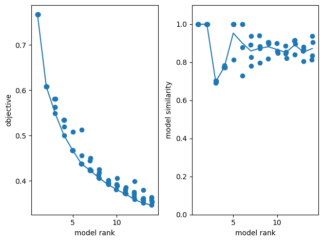
rank = 6
during_training_model = fit_shifted_cp(
spikes_tensor,
rank=rank,
boundary="wrap",
# n_restarts=N_RESTARTS,
n_restarts=10,
max_shift_axis0=MAX_SHIFT,
max_shift_axis1=None,
max_iter=100,
u_nonneg=True,
v_nonneg=True,
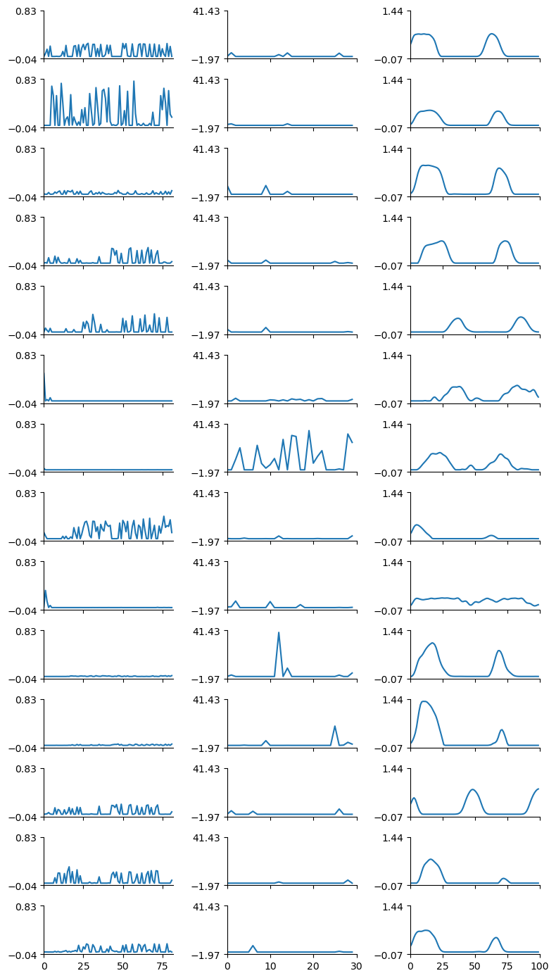
)fig = plot_result_with_ipd_coloring(
during_training_model, recorded_ipds, vertical_layout=True
)
# plt.show()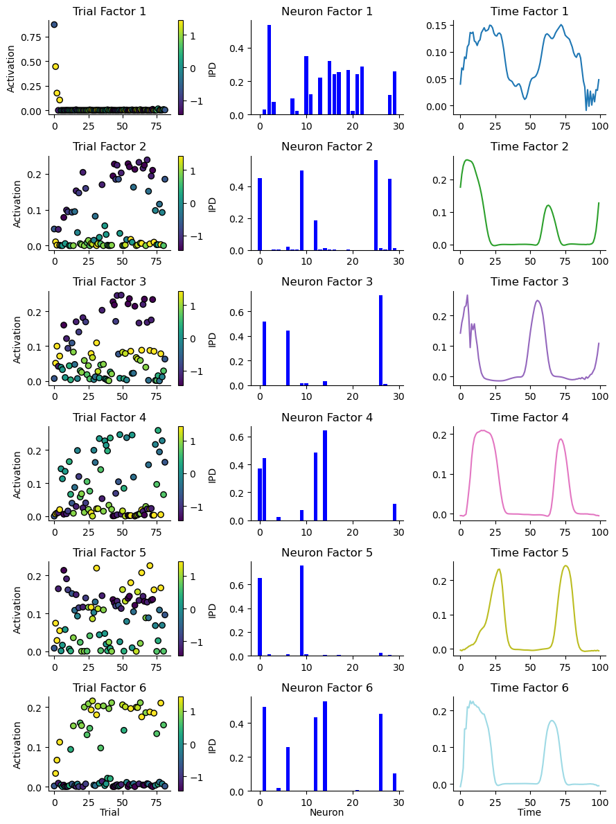
# Rank 1 model
during_training_model1 = fit_shifted_cp(
    spikes_tensor,
    rank=1,
    boundary="wrap",
    # n_restarts=N_RESTARTS,
    n_restarts=10,
    max_shift_axis0=MAX_SHIFT,
    max_shift_axis1=None,
    max_iter=100,
    u_nonneg=True,
    v_nonneg=True,
)

fig = plot_result_with_ipd_coloring(
    during_training_model1, recorded_ipds, vertical_layout=True
)
# fig.suptitle("Shifted Tensor Decomposition")
# plt.show()

plt.savefig(str(fig_counter) + '.png', dpi=300)
plt.savefig(str(fig_counter) + '.tiff', dpi=300)
fig_counter += 1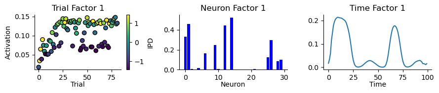
Evaluation post-training:
# Single IPD dataset
def non_random_ipd_input_signal(num_samples, bin=1, tensor=True):
    # ipd = (
    #     np.random.rand(num_samples) * np.pi - np.pi / 2
    # )  # uniformly random in (-pi/2, pi/2)
    # generate a set of ipds that are all the same
    # ipd = np.repeat(ipd, num_samples)
    # generate ipds that fall within the class range
    ipd = continuise(bin)
    ipd = np.repeat(ipd, num_samples)
    # add noise to ipds of 7.5 degrees
    ipd = ipd + np.random.uniform(-np.pi / 24, np.pi / 24, size=ipd.shape)

    spikes = input_signal(ipd)
    if tensor:
        ipd = torch.tensor(ipd, device=device, dtype=dtype)
        spikes = torch.tensor(spikes, device=device, dtype=dtype)
    return ipd, spikes


# Plot a few just to show how it looks
# bins range from 0 - 11
bin = 5
ipd, spikes = non_random_ipd_input_signal(8, bin=11)  # 6 is 0+15 degrees
spikes_plot = spikes.cpu()
plt.figure(figsize=(10, 4), dpi=100)
for i in range(8):
    plt.subplot(2, 4, i + 1)
    plt.imshow(
        spikes_plot[i, :, :].T,
        aspect="auto",
        interpolation="nearest",
        cmap=plt.cm.gray_r,
    )
    plt.title(f"True IPD = {int(ipd[i]*180/np.pi)} deg")
    if i >= 4:
        plt.xlabel("Time (steps)")
    if i % 4 == 0:
        plt.ylabel("Input neuron index")
plt.tight_layout()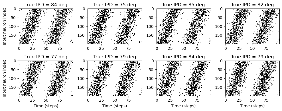
def evaluate_full_ipd_range(ipds, spikes, model):
    """
    This function evaluates a model across the full range of IPD values and collects the output spikes
    and estimated IPDs.
    """
    spike_data = []
    ipd_data = []
    estimated_ipd_data = []

    # Generate data in batches and evaluate
    for x_local, y_local in data_generator(discretise(ipds), spikes, random=False):
        # Run the model to get output spikes and membrane potentials
        output = model(x_local)
        output_spikes, output_vrec = output

        # Compute the estimated IPDs from the output membrane potentials
        _, estimated_ipds = torch.max(
            output_vrec, dim=1
        )  # Ensure you specify the dimension if needed

        # get the estimated ipds as a list of categories
        estimated_ipds = estimated_ipds.cpu().detach().numpy()
        # convert from [4096, 12] to [4096]
        estimated_ipds = np.argmax(estimated_ipds, axis=1)

        # Collect output spikes, true IPD values, and estimated IPD values
        spike_data.append(output_spikes.detach().cpu().numpy())
        ipd_data.append(y_local.detach().cpu().numpy())
        estimated_ipd_data.append(estimated_ipds)

    # Convert list to tensors
    spikes_tensor = torch.tensor(np.concatenate(spike_data), dtype=torch.float32)
    ipd_tensor = torch.tensor(np.concatenate(ipd_data), dtype=torch.float32)
    estimated_ipd_tensor = torch.tensor(
        np.concatenate(estimated_ipd_data), dtype=torch.int64
    )

    return spikes_tensor, ipd_tensor, estimated_ipd_tensor


print(f"Chance accuracy level: {100*1/num_classes:.1f}%")
snn_model = lambda x: snn(x, W1, W2)
Chance accuracy level: 8.3%
# Single IPD
# ipd, spikes = non_random_ipd_input_signal(num_samples, bin=bin)
# Normal random IPD
# ipd, spikes = random_ipd_input_signal(num_samples)
# Ordered IPDs
ipd, spikes = random_step_ipd_input_signal(num_samples)

print("spikes shape: ", spikes.shape)
output_spikes_test, output_ipds_test, output_est_ipds = evaluate_full_ipd_range(
    ipd, spikes, snn_model
)

print("Output spikes test shape:", output_spikes_test.shape)
print("Output IPDs test shape:", output_ipds_test.shape)
print("Output estimated IPDs shape:", output_est_ipds.shape)

output_ipds_test_pca = output_ipds_test.detach().cpu().numpy().astype(np.float64)
output_est_ipds_pca = output_est_ipds.detach().cpu().numpy().astype(np.float64)

# create a vecctor with 0 and 1 for correct and incorrect predictions
correct_predictions = (output_ipds_test_pca == output_est_ipds_pca).astype(int)
incorrect_predictions = (output_ipds_test_pca != output_est_ipds_pca).astype(int)
print("Number of correct predictions:", np.sum(correct_predictions))
print("Number of incorrect predictions:", np.sum(incorrect_predictions))
spikes shape: torch.Size([4096, 100, 200])
Output spikes test shape: torch.Size([4096, 100, 30])
Output IPDs test shape: torch.Size([4096])
Output estimated IPDs shape: torch.Size([4096])
Number of correct predictions: 722
Number of incorrect predictions: 3374
def transform_eval_spikes(recorded_spikes, sigma=2.0):
    # Convert to num samples, neurons, time
    reshaped_spikes = recorded_spikes.permute(0, 2, 1).cpu().numpy().astype(np.float64)

    # Apply Gaussian smoothing along the time axis for each neuron
    smoothed_spikes = np.zeros_like(reshaped_spikes)
    for i in range(reshaped_spikes.shape[0]):
        for j in range(reshaped_spikes.shape[1]):
            smoothed_spikes[i, j, :] = gaussian_filter1d(
                reshaped_spikes[i, j, :], sigma=sigma
            )

    return smoothed_spikes
output_spikes_test = transform_eval_spikes(output_spikes_test)
output_ipds_test = (
output_ipds_test.view(-1).detach().cpu().numpy().astype(np.float64).flatten()
)
print("Output spikes test shape:", output_spikes_test.shape)
print("Output IPDs test shape:", output_ipds_test.shape)
# Reduce the size of the spikes_tensor, recorded_ipds and recorded_estimated_ipds by sampling every 10th sample
divide_by = 10
output_spikes_test = output_spikes_test[::divide_by]
output_ipds_test = output_ipds_test[::divide_by]
print("Output spikes test shape:", output_spikes_test.shape)
print("Output IPDs test shape:", output_ipds_test.shape)Output spikes test shape: (4096, 30, 100)
Output IPDs test shape: (4096,)
Output spikes test shape: (410, 30, 100)
Output IPDs test shape: (410,)
# test up to 18 components
num_components = 18

# Fit an ensemble of models, 4 random replicates / optimization runs per model rank
ensemble = tt.Ensemble(fit_method="ncp_hals")
ensemble.fit(
    output_spikes_test, ranks=range(1, num_components), replicates=5
)  # range(1,32)
# list of numbers from 1 to 40 in steps of 5 range(7, 10, 2)

fig, axes = plt.subplots(1, 2)
# plot reconstruction error as a function of num components.
tt.plot_objective(ensemble, ax=axes[0])
# plot model similarity as a function of num components.
tt.plot_similarity(ensemble, ax=axes[1])
fig.tight_layout()

# Plot the low-d factors =
replicate = 0
tt.plot_factors(
    ensemble.factors(num_components - 1)[replicate]
)  # plot the low-d factors

# plt.show()
Rank-1 models: min obj, 0.73; max obj, 0.73; time to fit, 0.5s
Rank-2 models: min obj, 0.57; max obj, 0.57; time to fit, 0.7s
Rank-3 models: min obj, 0.49; max obj, 0.52; time to fit, 0.9s
Rank-4 models: min obj, 0.44; max obj, 0.46; time to fit, 1.5s
Rank-5 models: min obj, 0.40; max obj, 0.42; time to fit, 3.5s
Rank-6 models: min obj, 0.38; max obj, 0.41; time to fit, 3.9s
Rank-7 models: min obj, 0.36; max obj, 0.41; time to fit, 4.6s
Rank-8 models: min obj, 0.35; max obj, 0.37; time to fit, 4.5s
Rank-9 models: min obj, 0.33; max obj, 0.37; time to fit, 3.4s
Rank-10 models: min obj, 0.33; max obj, 0.37; time to fit, 4.0s
Rank-11 models: min obj, 0.31; max obj, 0.36; time to fit, 3.9s
Rank-12 models: min obj, 0.30; max obj, 0.33; time to fit, 4.4s
Rank-13 models: min obj, 0.30; max obj, 0.34; time to fit, 5.0s
Rank-14 models: min obj, 0.29; max obj, 0.32; time to fit, 6.6s
Rank-15 models: min obj, 0.29; max obj, 0.31; time to fit, 6.4s
Rank-16 models: min obj, 0.29; max obj, 0.31; time to fit, 5.7s
Rank-17 models: min obj, 0.29; max obj, 0.30; time to fit, 5.9s
(<Figure size 800x1700 with 51 Axes>,
 array([[<AxesSubplot: >, <AxesSubplot: >, <AxesSubplot: >],
        [<AxesSubplot: >, <AxesSubplot: >, <AxesSubplot: >],
        [<AxesSubplot: >, <AxesSubplot: >, <AxesSubplot: >],
        [<AxesSubplot: >, <AxesSubplot: >, <AxesSubplot: >],
        [<AxesSubplot: >, <AxesSubplot: >, <AxesSubplot: >],
        [<AxesSubplot: >, <AxesSubplot: >, <AxesSubplot: >],
        [<AxesSubplot: >, <AxesSubplot: >, <AxesSubplot: >],
        [<AxesSubplot: >, <AxesSubplot: >, <AxesSubplot: >],
        [<AxesSubplot: >, <AxesSubplot: >, <AxesSubplot: >],
        [<AxesSubplot: >, <AxesSubplot: >, <AxesSubplot: >],
        [<AxesSubplot: >, <AxesSubplot: >, <AxesSubplot: >],
        [<AxesSubplot: >, <AxesSubplot: >, <AxesSubplot: >],
        [<AxesSubplot: >, <AxesSubplot: >, <AxesSubplot: >],
        [<AxesSubplot: >, <AxesSubplot: >, <AxesSubplot: >],
        [<AxesSubplot: >, <AxesSubplot: >, <AxesSubplot: >],
        [<AxesSubplot: >, <AxesSubplot: >, <AxesSubplot: >],
        [<AxesSubplot: >, <AxesSubplot: >, <AxesSubplot: >]], dtype=object),
 array([[list([<matplotlib.lines.Line2D object at 0x0000019E1BF2B340>]),
         list([<matplotlib.lines.Line2D object at 0x0000019E1BF60F10>]),
         list([<matplotlib.lines.Line2D object at 0x0000019E1BF62350>])],
        [list([<matplotlib.lines.Line2D object at 0x0000019E1BF74AF0>]),
         list([<matplotlib.lines.Line2D object at 0x0000019E1BF75CF0>]),
         list([<matplotlib.lines.Line2D object at 0x0000019E1BF74160>])],
        [list([<matplotlib.lines.Line2D object at 0x0000019E1BF8D8D0>]),
         list([<matplotlib.lines.Line2D object at 0x0000019E1BF8EBF0>]),
         list([<matplotlib.lines.Line2D object at 0x0000019E1BF8C760>])],
        [list([<matplotlib.lines.Line2D object at 0x0000019E1BFAE6B0>]),
         list([<matplotlib.lines.Line2D object at 0x0000019E1BFAFAF0>]),
         list([<matplotlib.lines.Line2D object at 0x0000019E1BFC4D60>])],
        [list([<matplotlib.lines.Line2D object at 0x0000019E1BFC75B0>]),
         list([<matplotlib.lines.Line2D object at 0x0000019E1BFE4400>]),
         list([<matplotlib.lines.Line2D object at 0x0000019E1BFE60B0>])],
        [list([<matplotlib.lines.Line2D object at 0x0000019E1BFE7CD0>]),
         list([<matplotlib.lines.Line2D object at 0x0000019E1BFFD150>]),
         list([<matplotlib.lines.Line2D object at 0x0000019E1BFFEE00>])],
        [list([<matplotlib.lines.Line2D object at 0x0000019E1C01CC10>]),
         list([<matplotlib.lines.Line2D object at 0x0000019E1C01DF30>]),
         list([<matplotlib.lines.Line2D object at 0x0000019E1C01FBE0>])],
        [list([<matplotlib.lines.Line2D object at 0x0000019E1C035B10>]),
         list([<matplotlib.lines.Line2D object at 0x0000019E1C036E30>]),
         list([<matplotlib.lines.Line2D object at 0x0000019E1C058B20>])],
        [list([<matplotlib.lines.Line2D object at 0x0000019E1C05AA10>]),
         list([<matplotlib.lines.Line2D object at 0x0000019E1C05BD30>]),
         list([<matplotlib.lines.Line2D object at 0x0000019E1C071A20>])],
        [list([<matplotlib.lines.Line2D object at 0x0000019E1C073910>]),
         list([<matplotlib.lines.Line2D object at 0x0000019E1C08CC70>]),
         list([<matplotlib.lines.Line2D object at 0x0000019E1C08E920>])],
        [list([<matplotlib.lines.Line2D object at 0x0000019E1C0A4850>]),
         list([<matplotlib.lines.Line2D object at 0x0000019E1C0A4EB0>]),
         list([<matplotlib.lines.Line2D object at 0x0000019E1C0A6FB0>])],
        [list([<matplotlib.lines.Line2D object at 0x0000019E1C0C0F10>]),
         list([<matplotlib.lines.Line2D object at 0x0000019E1C0C2110>]),
         list([<matplotlib.lines.Line2D object at 0x0000019E1C0C3DC0>])],
        [list([<matplotlib.lines.Line2D object at 0x0000019E1C0DDCF0>]),
         list([<matplotlib.lines.Line2D object at 0x0000019E1C0DC8E0>]),
         list([<matplotlib.lines.Line2D object at 0x0000019E1C0F4D00>])],
        [list([<matplotlib.lines.Line2D object at 0x0000019E1C0F6C80>]),
         list([<matplotlib.lines.Line2D object at 0x0000019E1C0F4490>]),
         list([<matplotlib.lines.Line2D object at 0x0000019E1C111DB0>])],
        [list([<matplotlib.lines.Line2D object at 0x0000019E1C113D30>]),
         list([<matplotlib.lines.Line2D object at 0x0000019E1C1348B0>]),
         list([<matplotlib.lines.Line2D object at 0x0000019E1C136DD0>])],
        [list([<matplotlib.lines.Line2D object at 0x0000019E1C144D90>]),
         list([<matplotlib.lines.Line2D object at 0x0000019E1C145510>]),
         list([<matplotlib.lines.Line2D object at 0x0000019E1C147D60>])],
        [list([<matplotlib.lines.Line2D object at 0x0000019E1C165C90>]),
         list([<matplotlib.lines.Line2D object at 0x0000019E1C1663E0>]),
         list([<matplotlib.lines.Line2D object at 0x0000019E1C166B30>])]],
       dtype=object))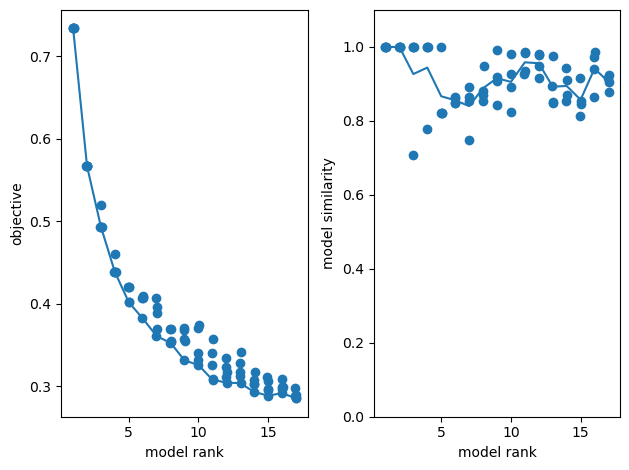
eval_testing_model = fit_shifted_cp(
output_spikes_test,
rank=1,
boundary="wrap",
n_restarts=N_RESTARTS,
max_shift_axis0=MAX_SHIFT,
max_shift_axis1=None,
max_iter=100,
u_nonneg=False,
v_nonneg=True,
)
# Plot a few raster plots of output_spikes_test ([4096, 100, 30])
fig, axs = plt.subplots(1, 4, figsize=(20, 5))
for i in range(4):
axs[i].imshow(
output_spikes_test[i, :, :],
aspect="auto",
interpolation="nearest",
cmap=plt.cm.gray_r,
)
axs[i].set_title(f"True IPD = {output_ipds_test[i]} deg")
axs[i].set_xlabel("Time (steps)")
axs[i].set_ylabel("Output neuron index")
plt.tight_layout()
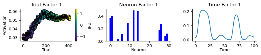
# Example usage assuming model is defined and appropriate
fig = plot_result_with_ipd_coloring(
eval_testing_model, output_ipds_test, vertical_layout=True
)
# fig.suptitle("Shifted Tensor Decomposition")
# plt.show()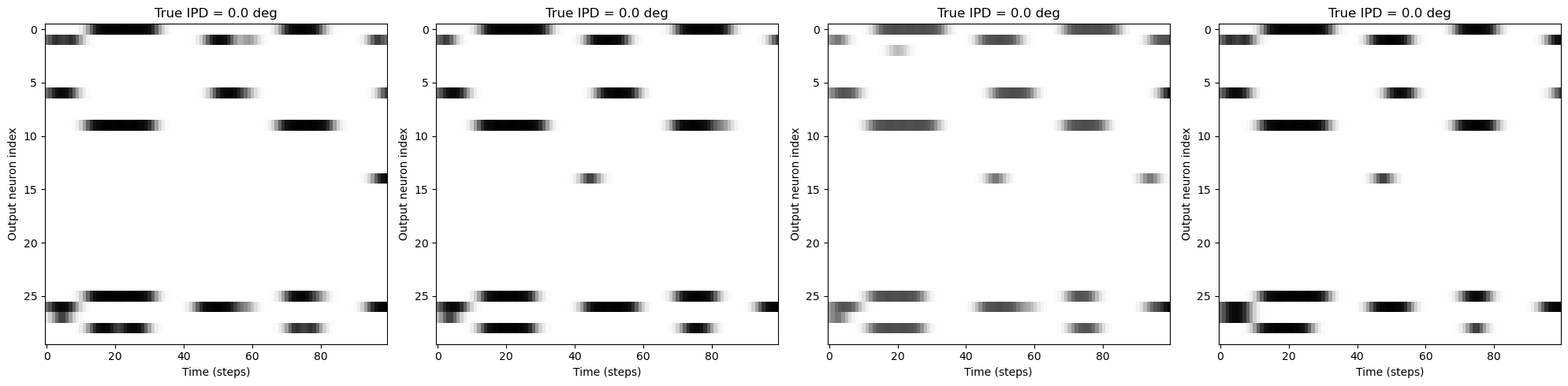
eval_testing_model = fit_shifted_cp(
    output_spikes_test,
    rank=rank,
    boundary="wrap",
    n_restarts=N_RESTARTS,
    max_shift_axis0=MAX_SHIFT,
    max_shift_axis1=None,
    max_iter=100,
    u_nonneg=False,
    v_nonneg=True,
)

# Plot a few raster plots of output_spikes_test ([4096, 100, 30])
fig, axs = plt.subplots(1, 4, figsize=(20, 5))
for i in range(4):
    axs[i].imshow(
        output_spikes_test[i, :, :],
        aspect="auto",
        interpolation="nearest",
        cmap=plt.cm.gray_r,
    )
    axs[i].set_title(f"True IPD = {output_ipds_test[i]} deg")
    axs[i].set_xlabel("Time (steps)")
    axs[i].set_ylabel("Output neuron index")
plt.tight_layout()

# Example usage assuming model is defined and appropriate
fig = plot_result_with_ipd_coloring(
    eval_testing_model, output_ipds_test, vertical_layout=True
)
# fig.suptitle("Shifted Tensor Decomposition")
# plt.show()

plt.savefig(str(fig_counter) + '.png', dpi=300)
plt.savefig(str(fig_counter) + '.tiff', dpi=300)
fig_counter += 1
import concurrent.futures
import pandas as pd
def train_and_evaluate(ipds, spikes, nb_epochs, lr, num_classes, rank, batch_function):
W1, W2, recorded_spikes, recorded_input_ipds, recorded_estimated_ipds = (
train_network(ipds, spikes, nb_epochs, lr, num_classes)
)
spikes_tensor = transform_spikes(recorded_spikes)
spikes_tensor = spikes_tensor[::500]
during_training_model = fit_shifted_cp(
spikes_tensor,
rank=rank,
boundary="wrap",
n_restarts=10,
max_shift_axis0=MAX_SHIFT,
max_iter=100,
u_nonneg=True,
v_nonneg=True,
)
output_spikes_test, output_ipds_test, output_est_ipds = evaluate_full_ipd_range(
ipds, spikes, lambda x: snn(x, W1, W2)
)
output_spikes_test = transform_eval_spikes(output_spikes_test)[::10]
eval_testing_model = fit_shifted_cp(
output_spikes_test,
rank=rank,
boundary="wrap",
n_restarts=10,
max_shift_axis0=MAX_SHIFT,
max_iter=100,
u_nonneg=False,
v_nonneg=True,
)
train_accuracy = analyse(ipds, spikes, "Train", lambda x: snn(x, W1, W2)[-1])
ipds_test, spikes_test = random_ipd_input_signal(num_samples)
test_accuracy = analyse(
ipds_test, spikes_test, "Test", lambda x: snn(x, W1, W2)[-1]
)
return (during_training_model, eval_testing_model, train_accuracy, test_accuracy)
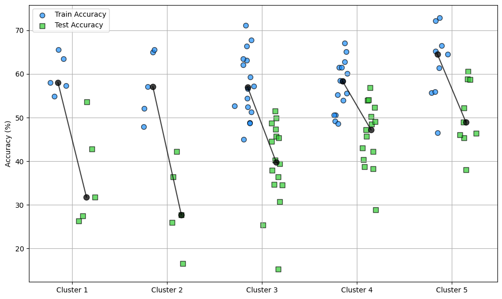
def run_multiple_experiments(
num_trials, ipds, spikes, nb_epochs, lr, num_classes, rank, batch_function
):
results = []
accuracies = []
with concurrent.futures.ThreadPoolExecutor(max_workers=5) as executor:
futures = [
executor.submit(
train_and_evaluate,
ipds,
spikes,
nb_epochs,
lr,
num_classes,
rank,
batch_function,
)
for _ in range(num_trials)
]
for future in concurrent.futures.as_completed(futures):
try:
result = future.result()
results.append(result[:2]) # Store models
accuracies.append(
{"Train Accuracy": result[2], "Test Accuracy": result[3]}
)
except Exception as e:
print(f"An error occurred: {e}")
# Optionally handle the failed case or retry
df_accuracies = pd.DataFrame(accuracies)
return results, df_accuracies
nb_epochs = 10
lr = 0.01
rank = 1
num_samples = 1000
ipds, spikes = random_ipd_input_signal(num_samples)
results, accuracies = run_multiple_experiments(
50, ipds, spikes, nb_epochs, lr, num_classes, rank, data_generator
)
print(accuracies)Epoch 1: loss=3.11377
Epoch 1: loss=2.89105
Epoch 1: loss=2.90078
Epoch 1: loss=2.46854
Epoch 1: loss=3.05766
Epoch 2: loss=2.32668
Epoch 2: loss=2.44810
Epoch 2: loss=2.36071
Epoch 2: loss=1.96940
Epoch 2: loss=2.43808
Epoch 3: loss=2.05225
Epoch 3: loss=2.26865
Epoch 3: loss=1.74541
Epoch 3: loss=2.17384
Epoch 3: loss=2.21912
Epoch 4: loss=1.79359
Epoch 4: loss=2.08371
Epoch 4: loss=1.57007
Epoch 4: loss=2.00098
Epoch 4: loss=2.06220
Epoch 5: loss=1.63325
Epoch 5: loss=1.42433
Epoch 5: loss=1.86919
Epoch 5: loss=1.83351
Epoch 5: loss=1.92643
Epoch 6: loss=1.50094
Epoch 6: loss=1.32022
Epoch 6: loss=1.70417
Epoch 6: loss=1.69419
Epoch 6: loss=1.79937
Epoch 7: loss=1.39539
Epoch 7: loss=1.21880
Epoch 7: loss=1.56884
Epoch 7: loss=1.54022
Epoch 7: loss=1.69048
Epoch 8: loss=1.35050
Epoch 8: loss=1.15821
Epoch 8: loss=1.46068
Epoch 8: loss=1.42274
Epoch 8: loss=1.59521
Epoch 9: loss=1.26652
Epoch 9: loss=1.07188
Epoch 9: loss=1.38108
Epoch 9: loss=1.32133
Epoch 9: loss=1.52436
Epoch 10: loss=1.03926
Epoch 10: loss=1.21450
Epoch 10: loss=1.30459
Epoch 10: loss=1.22729
Epoch 10: loss=1.45547
Train classifier accuracy: 72.9%
Train absolute error: 5.8 deg
Train classifier accuracy: 54.4%
Train absolute error: 9.7 deg
Train classifier accuracy: 56.7%
Train absolute error: 8.4 deg
Train classifier accuracy: 71.1%
Train absolute error: 5.9 deg
Train classifier accuracy: 48.9%
Train absolute error: 12.1 deg
Test classifier accuracy: 60.6%
Test absolute error: 7.2 deg
Test classifier accuracy: 47.3%
Test absolute error: 10.1 deg
Test classifier accuracy: 49.9%
Test absolute error: 9.0 deg
Test classifier accuracy: 34.7%
Test absolute error: 13.5 deg
Test classifier accuracy: 36.4%
Test absolute error: 13.5 deg
Epoch 1: loss=2.81427
Epoch 1: loss=2.93173
Epoch 1: loss=2.81124
Epoch 1: loss=2.78725
Epoch 1: loss=2.95713
Epoch 2: loss=2.32325
Epoch 2: loss=2.32537
Epoch 2: loss=2.34727
Epoch 2: loss=2.24539
Epoch 2: loss=2.17843
Epoch 3: loss=2.08903
Epoch 3: loss=2.16320
Epoch 3: loss=2.05495
Epoch 3: loss=2.04131
Epoch 3: loss=1.95081
Epoch 4: loss=1.88597
Epoch 4: loss=1.99126
Epoch 4: loss=1.84940
Epoch 4: loss=1.86924
Epoch 4: loss=1.75070
Epoch 5: loss=1.72124
Epoch 5: loss=1.77983
Epoch 5: loss=1.68358
Epoch 5: loss=1.72849
Epoch 5: loss=1.57830
Epoch 6: loss=1.59135
Epoch 6: loss=1.59012
Epoch 6: loss=1.57593
Epoch 6: loss=1.61668
Epoch 6: loss=1.43507
Epoch 7: loss=1.46839
Epoch 7: loss=1.45284
Epoch 7: loss=1.48347
Epoch 7: loss=1.50776
Epoch 7: loss=1.33447
Epoch 8: loss=1.36997
Epoch 8: loss=1.36228
Epoch 8: loss=1.39509
Epoch 8: loss=1.42378
Epoch 8: loss=1.23835
Epoch 9: loss=1.28574
Epoch 9: loss=1.27352
Epoch 9: loss=1.34705
Epoch 9: loss=1.35551
Epoch 9: loss=1.16167
Epoch 10: loss=1.20055
Epoch 10: loss=1.21249
Epoch 10: loss=1.24865
Epoch 10: loss=1.31067
Epoch 10: loss=1.09185
Train classifier accuracy: 58.3%
Train absolute error: 8.3 deg
Test classifier accuracy: 50.2%
Test absolute error: 9.3 deg
Train classifier accuracy: 65.0%
Train absolute error: 7.4 deg
Epoch 1: loss=3.00438
Train classifier accuracy: 49.2%
Train absolute error: 10.7 deg
No artists with labels found to put in legend. Note that artists whose label start with an underscore are ignored when legend() is called with no argument.
Test classifier accuracy: 27.7%
Test absolute error: 29.2 deg

Train classifier accuracy: 51.2%
Train absolute error: 9.5 deg

Train classifier accuracy: 54.0%
Train absolute error: 8.7 deg

Test classifier accuracy: 40.3%
Test absolute error: 11.4 deg

Test classifier accuracy: 30.7%
Test absolute error: 20.3 deg

Test classifier accuracy: 48.5%
Test absolute error: 10.0 deg
Epoch 2: loss=2.22856
Epoch 1: loss=2.89430
Epoch 1: loss=3.23630
Epoch 1: loss=2.73547
Epoch 1: loss=2.99345
Epoch 3: loss=2.00344
Epoch 2: loss=2.37381
Epoch 2: loss=2.31116
Epoch 2: loss=2.32296
Epoch 2: loss=2.31411
Epoch 4: loss=1.83832
Epoch 3: loss=2.09775
Epoch 3: loss=2.07337
Epoch 3: loss=2.03755
Epoch 3: loss=2.04587
Epoch 5: loss=1.72534
Epoch 4: loss=1.91412
Epoch 4: loss=1.89178
Epoch 4: loss=1.81126
Epoch 4: loss=1.82214
Epoch 6: loss=1.63971
Epoch 5: loss=1.79666
Epoch 5: loss=1.74913
Epoch 5: loss=1.66020
Epoch 5: loss=1.64792
Epoch 7: loss=1.55785
Epoch 6: loss=1.69438
Epoch 6: loss=1.66673
Epoch 6: loss=1.50126
Epoch 6: loss=1.49119
Epoch 8: loss=1.47937
Epoch 7: loss=1.57150
Epoch 7: loss=1.57128
Epoch 7: loss=1.35217
Epoch 7: loss=1.37274
Epoch 9: loss=1.39667
Epoch 8: loss=1.45384
Epoch 8: loss=1.50403
Epoch 8: loss=1.26140
Epoch 8: loss=1.29640
Epoch 10: loss=1.33114
Epoch 9: loss=1.35049
Epoch 9: loss=1.42369
Epoch 9: loss=1.15976
Epoch 9: loss=1.21224
Epoch 10: loss=1.26771
Epoch 10: loss=1.33981
Epoch 10: loss=1.07011
Epoch 10: loss=1.15589

Train classifier accuracy: 52.7%
Train absolute error: 8.5 deg
C:\Users\ghosh\AppData\Local\Temp\ipykernel_30480\2324308904.py:25: RuntimeWarning: More than 20 figures have been opened. Figures created through the pyplot interface (`matplotlib.pyplot.figure`) are retained until explicitly closed and may consume too much memory. (To control this warning, see the rcParam `figure.max_open_warning`). Consider using `matplotlib.pyplot.close()`.
  plt.figure(figsize=(10, 4), dpi=100)
Test classifier accuracy: 25.3%
Test absolute error: 18.1 deg
Epoch 1: loss=2.80883
Epoch 2: loss=2.44840

Train classifier accuracy: 61.5%
Train absolute error: 7.6 deg

Train classifier accuracy: 50.6%
Train absolute error: 11.4 deg

Train classifier accuracy: 72.2%
Train absolute error: 5.9 deg

Train classifier accuracy: 61.6%
Train absolute error: 7.7 deg

Test classifier accuracy: 54.0%
Test absolute error: 8.5 deg

Test classifier accuracy: 38.8%
Test absolute error: 14.2 deg

Test classifier accuracy: 45.3%
Test absolute error: 12.0 deg

Test classifier accuracy: 56.9%
Test absolute error: 7.6 deg
Epoch 3: loss=2.29577
Epoch 1: loss=2.65173
Epoch 1: loss=2.72050
Epoch 4: loss=2.05546
Epoch 1: loss=2.99131
Epoch 1: loss=2.88022
Epoch 2: loss=2.17829
Epoch 2: loss=2.34290
Epoch 5: loss=1.80616
Epoch 2: loss=2.17002
Epoch 2: loss=2.16466
Epoch 3: loss=1.90002
Epoch 3: loss=2.17070
Epoch 6: loss=1.65046
Epoch 3: loss=1.84308
Epoch 3: loss=1.92668
Epoch 4: loss=1.65687
Epoch 4: loss=2.04231
Epoch 7: loss=1.52178
Epoch 4: loss=1.59441
Epoch 4: loss=1.77824
Epoch 5: loss=1.51320
Epoch 5: loss=1.93743
Epoch 8: loss=1.42789
Epoch 5: loss=1.42806
Epoch 5: loss=1.70014
Epoch 6: loss=1.40606
Epoch 6: loss=1.82892
Epoch 9: loss=1.34193
Epoch 6: loss=1.32168
Epoch 6: loss=1.61417
Epoch 10: loss=1.25937
Epoch 7: loss=1.30302
Epoch 7: loss=1.73520
Epoch 7: loss=1.25476
Epoch 7: loss=1.56416
Epoch 8: loss=1.20160
Epoch 8: loss=1.66602
Epoch 8: loss=1.17916
Epoch 8: loss=1.49206
Epoch 9: loss=1.13835
Epoch 9: loss=1.55196
Epoch 9: loss=1.11602
Epoch 9: loss=1.42624
Epoch 10: loss=1.08459
Epoch 10: loss=1.46615
Epoch 10: loss=1.08171
Epoch 10: loss=1.38291

Train classifier accuracy: 65.5%
Train absolute error: 6.9 deg

Test classifier accuracy: 53.6%
Test absolute error: 8.3 deg
Epoch 1: loss=2.80042
Epoch 2: loss=2.26626
Epoch 3: loss=2.01625
Epoch 4: loss=1.82557
Epoch 5: loss=1.64347

Train classifier accuracy: 47.9%
Train absolute error: 9.8 deg

Train classifier accuracy: 65.2%
Train absolute error: 7.2 deg
No artists with labels found to put in legend. Note that artists whose label start with an underscore are ignored when legend() is called with no argument.
Train classifier accuracy: 46.6%
Train absolute error: 10.9 deg

Train classifier accuracy: 67.8%
Train absolute error: 6.6 deg
C:\Users\ghosh\AppData\Local\Temp\ipykernel_30480\2324308904.py:33: MatplotlibDeprecationWarning: Auto-removal of overlapping axes is deprecated since 3.6 and will be removed two minor releases later; explicitly call ax.remove() as needed.
  plt.subplot(122)
Test classifier accuracy: 25.9%
Test absolute error: 48.2 deg
Epoch 6: loss=1.48167

Test classifier accuracy: 52.2%
Test absolute error: 9.7 deg

Test classifier accuracy: 39.4%
Test absolute error: 15.0 deg

Test classifier accuracy: 38.0%
Test absolute error: 12.9 deg
Epoch 7: loss=1.38756
Epoch 1: loss=2.78937
Epoch 1: loss=2.70414
Epoch 1: loss=2.70814
Epoch 1: loss=2.99843
Epoch 8: loss=1.28684
Epoch 2: loss=2.10455
Epoch 2: loss=2.27240
Epoch 2: loss=2.32707
Epoch 2: loss=2.25070
Epoch 9: loss=1.19765
Epoch 3: loss=1.82804
Epoch 3: loss=2.07043
Epoch 3: loss=2.09414
Epoch 3: loss=2.04704
Epoch 10: loss=1.13345
Epoch 4: loss=1.65867
Epoch 4: loss=1.93928
Epoch 4: loss=1.85967
Epoch 4: loss=1.88419
Epoch 5: loss=1.53844
Epoch 5: loss=1.85551
Epoch 5: loss=1.70207
Epoch 5: loss=1.77425
Epoch 6: loss=1.38842
Epoch 6: loss=1.77719
Epoch 6: loss=1.57682
Epoch 6: loss=1.65961
Epoch 7: loss=1.31063
Epoch 7: loss=1.69592

Train classifier accuracy: 61.4%
Train absolute error: 7.3 deg
Epoch 7: loss=1.47209
Epoch 7: loss=1.56103

Test classifier accuracy: 58.9%
Test absolute error: 7.5 deg
Epoch 8: loss=1.25603
Epoch 8: loss=1.61287
Epoch 8: loss=1.38224
Epoch 8: loss=1.45137
Epoch 1: loss=2.96992
Epoch 9: loss=1.16621
Epoch 9: loss=1.55678
Epoch 9: loss=1.30955
Epoch 9: loss=1.35344
Epoch 2: loss=2.33279
Epoch 10: loss=1.10019
Epoch 10: loss=1.49846
Epoch 10: loss=1.25819
Epoch 10: loss=1.27046
Epoch 3: loss=2.14241
Epoch 4: loss=1.90279
Epoch 5: loss=1.69531
Epoch 6: loss=1.49151
Epoch 7: loss=1.34532
Epoch 8: loss=1.24049
Epoch 9: loss=1.13108

Train classifier accuracy: 62.1%
Train absolute error: 7.9 deg

Train classifier accuracy: 52.1%
Train absolute error: 8.9 deg

Train classifier accuracy: 57.1%
Train absolute error: 8.9 deg

Train classifier accuracy: 57.3%
Train absolute error: 7.8 deg

Test classifier accuracy: 48.8%
Test absolute error: 10.0 deg
Epoch 10: loss=1.06542

Test classifier accuracy: 36.5%
Test absolute error: 25.0 deg

Test classifier accuracy: 42.2%
Test absolute error: 13.0 deg

Test classifier accuracy: 31.8%
Test absolute error: 17.2 deg
Epoch 1: loss=2.97617
Epoch 1: loss=3.04330
Epoch 1: loss=3.09316
Epoch 1: loss=2.93614
Epoch 2: loss=2.25105
Epoch 2: loss=2.34976
Epoch 2: loss=2.28771
Epoch 2: loss=2.35784
Epoch 3: loss=1.94623

Train classifier accuracy: 63.1%
Train absolute error: 7.0 deg
Epoch 3: loss=2.09297
Epoch 3: loss=2.02376
Epoch 3: loss=2.16836

Test classifier accuracy: 51.6%
Test absolute error: 9.6 deg
Epoch 4: loss=1.70660
Epoch 4: loss=1.85280
Epoch 4: loss=1.84607
Epoch 4: loss=2.00161
Epoch 1: loss=3.06801
Epoch 5: loss=1.50320
Epoch 5: loss=1.65288
Epoch 5: loss=1.67303
Epoch 5: loss=1.88362
Epoch 2: loss=2.22444
Epoch 6: loss=1.35062
Epoch 6: loss=1.52017
Epoch 6: loss=1.54680
Epoch 3: loss=1.92982
Epoch 6: loss=1.77309
Epoch 7: loss=1.23884
Epoch 7: loss=1.39062
Epoch 7: loss=1.45870
Epoch 4: loss=1.73196
Epoch 7: loss=1.67439
Epoch 8: loss=1.16819
Epoch 8: loss=1.29842
Epoch 8: loss=1.35700
Epoch 5: loss=1.55928
Epoch 8: loss=1.59086
Epoch 9: loss=1.10261
Epoch 9: loss=1.22334
Epoch 6: loss=1.40921
Epoch 9: loss=1.30080
Epoch 9: loss=1.55393
Epoch 10: loss=1.01161
Epoch 10: loss=1.17160
Epoch 7: loss=1.28293
Epoch 10: loss=1.23209
Epoch 10: loss=1.46983
Epoch 8: loss=1.18226
Epoch 9: loss=1.13230
Epoch 10: loss=1.09088

Train classifier accuracy: 67.1%
Train absolute error: 6.8 deg

Train classifier accuracy: 62.8%
Train absolute error: 7.4 deg

Test classifier accuracy: 42.2%
Test absolute error: 10.9 deg

Train classifier accuracy: 60.1%
Train absolute error: 7.6 deg

Test classifier accuracy: 38.2%
Test absolute error: 13.4 deg

Train classifier accuracy: 48.8%
Train absolute error: 12.1 deg

Test classifier accuracy: 28.9%
Test absolute error: 22.0 deg
Epoch 1: loss=2.93547

Test classifier accuracy: 15.2%
Test absolute error: 32.8 deg

Train classifier accuracy: 65.1%
Train absolute error: 6.7 deg
Epoch 1: loss=3.04972

Test classifier accuracy: 52.3%
Test absolute error: 9.0 deg
Epoch 1: loss=3.07396
Epoch 2: loss=2.44180
Epoch 1: loss=2.83590
Epoch 2: loss=2.40934
Epoch 1: loss=2.83109
Epoch 2: loss=2.21587
Epoch 3: loss=2.28676
Epoch 2: loss=2.36715
Epoch 3: loss=2.17374
Epoch 2: loss=2.27092
Epoch 3: loss=1.93531
Epoch 4: loss=2.13252
Epoch 3: loss=2.16111
Epoch 4: loss=1.97270
Epoch 3: loss=2.01613
Epoch 4: loss=1.72168
Epoch 5: loss=1.96330
Epoch 4: loss=2.00198
Epoch 5: loss=1.79134
Epoch 4: loss=1.74456
Epoch 5: loss=1.55107
Epoch 6: loss=1.82634
Epoch 5: loss=1.87049
Epoch 6: loss=1.63445
Epoch 5: loss=1.53332
Epoch 6: loss=1.42346
Epoch 7: loss=1.70669
Epoch 6: loss=1.73680
Epoch 7: loss=1.50636
Epoch 6: loss=1.43123
Epoch 7: loss=1.33604
Epoch 8: loss=1.61543
Epoch 7: loss=1.60783
Epoch 8: loss=1.42933
Epoch 7: loss=1.33723
Epoch 8: loss=1.24676
Epoch 9: loss=1.52713
Epoch 8: loss=1.50321
Epoch 9: loss=1.36830
Epoch 8: loss=1.24458
Epoch 9: loss=1.18922
Epoch 10: loss=1.47164
Epoch 9: loss=1.40551
Epoch 10: loss=1.30864
Epoch 9: loss=1.18572
Epoch 10: loss=1.14626
Epoch 10: loss=1.32338
Epoch 10: loss=1.10434

Train classifier accuracy: 54.9%
Train absolute error: 9.2 deg
No artists with labels found to put in legend. Note that artists whose label start with an underscore are ignored when legend() is called with no argument.
Train classifier accuracy: 48.6%
Train absolute error: 10.2 deg

Test classifier accuracy: 27.5%
Test absolute error: 19.0 deg

Train classifier accuracy: 64.5%
Train absolute error: 7.1 deg

Test classifier accuracy: 45.7%
Test absolute error: 10.7 deg

Test classifier accuracy: 46.4%
Test absolute error: 10.0 deg

Train classifier accuracy: 55.7%
Train absolute error: 7.8 deg

Train classifier accuracy: 52.4%
Train absolute error: 9.5 deg
Epoch 1: loss=2.65049

Test classifier accuracy: 46.0%
Test absolute error: 9.3 deg

Test classifier accuracy: 45.7%
Test absolute error: 10.1 deg
Epoch 1: loss=3.21689
Epoch 1: loss=2.84275
Epoch 2: loss=2.27585
Epoch 1: loss=2.89037
Epoch 1: loss=2.92978
Epoch 2: loss=2.24485
Epoch 2: loss=2.21158
Epoch 3: loss=2.06614
Epoch 2: loss=2.31827
Epoch 2: loss=2.21600
Epoch 3: loss=1.93785
Epoch 3: loss=2.02922
Epoch 4: loss=1.83128
Epoch 3: loss=2.01695
Epoch 3: loss=1.98432
Epoch 4: loss=1.69173
Epoch 4: loss=1.87503
Epoch 5: loss=1.65337
Epoch 4: loss=1.79840
Epoch 4: loss=1.83687
Epoch 5: loss=1.51425
Epoch 5: loss=1.72561
Epoch 5: loss=1.66031
Epoch 6: loss=1.50706
Epoch 5: loss=1.71389
Epoch 6: loss=1.39689
Epoch 6: loss=1.59172
Epoch 6: loss=1.54791
Epoch 7: loss=1.39850
Epoch 6: loss=1.62435
Epoch 7: loss=1.27988
Epoch 7: loss=1.47240
Epoch 7: loss=1.45881
Epoch 8: loss=1.32580
Epoch 7: loss=1.52959
Epoch 8: loss=1.20809
Epoch 8: loss=1.38748
Epoch 8: loss=1.37445
Epoch 9: loss=1.24690
Epoch 8: loss=1.46361
Epoch 9: loss=1.13649
Epoch 9: loss=1.31181
Epoch 9: loss=1.30801
Epoch 10: loss=1.20239
Epoch 10: loss=1.08597
Epoch 9: loss=1.38105
Epoch 10: loss=1.24884
Epoch 10: loss=1.23911
Epoch 10: loss=1.32025

Train classifier accuracy: 66.6%
Train absolute error: 6.8 deg

Train classifier accuracy: 63.5%
Train absolute error: 7.1 deg

Test classifier accuracy: 58.8%
Test absolute error: 7.6 deg

Train classifier accuracy: 63.4%
Train absolute error: 7.4 deg

Test classifier accuracy: 42.8%
Test absolute error: 12.5 deg

Train classifier accuracy: 58.0%
Train absolute error: 8.2 deg

Test classifier accuracy: 44.6%
Test absolute error: 12.6 deg

Train classifier accuracy: 55.2%
Train absolute error: 8.5 deg

Test classifier accuracy: 26.4%
Test absolute error: 17.2 deg

Test classifier accuracy: 47.2%
Test absolute error: 9.4 deg
Epoch 1: loss=3.04166
Epoch 1: loss=2.65442
Epoch 1: loss=3.03546
Epoch 1: loss=3.12721
Epoch 1: loss=2.85149
Epoch 2: loss=2.43674
Epoch 2: loss=2.12722
Epoch 2: loss=2.32988
Epoch 2: loss=2.39052
Epoch 2: loss=2.35698
Epoch 3: loss=2.28889
Epoch 3: loss=1.88783
Epoch 3: loss=2.11076
Epoch 3: loss=2.14058
Epoch 3: loss=2.06612
Epoch 4: loss=2.12994
Epoch 4: loss=1.68690
Epoch 4: loss=1.93931
Epoch 4: loss=1.92603
Epoch 4: loss=1.88951
Epoch 5: loss=1.96327
Epoch 5: loss=1.52088
Epoch 5: loss=1.81723
Epoch 5: loss=1.75883
Epoch 5: loss=1.70228
Epoch 6: loss=1.82139
Epoch 6: loss=1.39351
Epoch 6: loss=1.73078
Epoch 6: loss=1.61982
Epoch 6: loss=1.57447
Epoch 7: loss=1.65871
Epoch 7: loss=1.31768
Epoch 7: loss=1.63048
Epoch 7: loss=1.54072
Epoch 7: loss=1.46482
Epoch 8: loss=1.54617
Epoch 8: loss=1.55358
Epoch 8: loss=1.24371
Epoch 8: loss=1.45055
Epoch 8: loss=1.37657
Epoch 9: loss=1.45241
Epoch 9: loss=1.48866
Epoch 9: loss=1.18574
Epoch 9: loss=1.36438
Epoch 9: loss=1.29095
Epoch 10: loss=1.37317
Epoch 10: loss=1.42575
Epoch 10: loss=1.14733
Epoch 10: loss=1.29265
Epoch 10: loss=1.23932

Train classifier accuracy: 50.6%
Train absolute error: 11.0 deg

Test classifier accuracy: 43.0%
Test absolute error: 12.7 deg

Train classifier accuracy: 57.2%
Train absolute error: 9.1 deg

Train classifier accuracy: 58.5%
Train absolute error: 7.8 deg

Train classifier accuracy: 59.3%
Train absolute error: 7.7 deg

Test classifier accuracy: 34.6%
Test absolute error: 14.7 deg

Train classifier accuracy: 55.9%
Train absolute error: 8.4 deg

Test classifier accuracy: 54.1%
Test absolute error: 8.5 deg

Test classifier accuracy: 45.3%
Test absolute error: 10.0 deg
Epoch 1: loss=2.52312

Test classifier accuracy: 49.0%
Test absolute error: 9.7 deg
Epoch 1: loss=3.14456
Epoch 1: loss=2.90721
Epoch 1: loss=2.48915
Epoch 2: loss=2.09500
Epoch 2: loss=2.40628
Epoch 2: loss=2.31444
Epoch 2: loss=2.12201
Epoch 3: loss=1.88967
Epoch 3: loss=2.10577
Epoch 3: loss=2.14980
Epoch 3: loss=1.85334
Epoch 4: loss=1.72403
Epoch 4: loss=1.92190
Epoch 4: loss=1.99069
Epoch 4: loss=1.61142
Epoch 5: loss=1.56953
Epoch 5: loss=1.78213
Epoch 5: loss=1.84999
Epoch 5: loss=1.42771
Epoch 6: loss=1.43410
Epoch 6: loss=1.66106
Epoch 6: loss=1.74828
Epoch 6: loss=1.28416
Epoch 7: loss=1.32094
Epoch 7: loss=1.53933
Epoch 7: loss=1.67032
Epoch 7: loss=1.17783
Epoch 8: loss=1.24271
Epoch 8: loss=1.47150
Epoch 8: loss=1.58993
Epoch 9: loss=1.16784
Epoch 8: loss=1.09145
Epoch 9: loss=1.40886
Epoch 10: loss=1.08752
Epoch 9: loss=1.52218
Epoch 9: loss=1.04248
Epoch 10: loss=1.32276
Epoch 10: loss=1.49398
Epoch 10: loss=0.97596

Train classifier accuracy: 66.4%
Train absolute error: 6.9 deg

Test classifier accuracy: 40.2%
Test absolute error: 13.4 deg

Train classifier accuracy: 65.5%
Train absolute error: 7.0 deg

Train classifier accuracy: 55.6%
Train absolute error: 8.2 deg

Test classifier accuracy: 16.6%
Test absolute error: 58.1 deg

Train classifier accuracy: 45.0%
Train absolute error: 11.4 deg

Test classifier accuracy: 49.1%
Test absolute error: 9.5 deg

Test classifier accuracy: 37.9%
Test absolute error: 12.7 deg
    Train Accuracy  Test Accuracy
0        72.916667      60.625000
1        54.375000      47.291667
2        56.666667      49.895833
3        71.145833      34.687500
4        48.854167      36.354167
5        58.333333      50.208333
6        65.000000      27.708333
7        49.166667      40.312500
8        51.250000      30.729167
9        53.958333      48.541667
10       52.708333      25.312500
11       61.458333      53.958333
12       50.625000      38.750000
13       72.187500      45.312500
14       61.562500      56.875000
15       65.520833      53.645833
16       47.916667      25.937500
17       65.208333      52.187500
18       67.812500      39.375000
19       46.562500      38.020833
20       61.354167      58.854167
21       62.083333      48.750000
22       52.083333      36.458333
23       57.083333      42.187500
24       57.291667      31.770833
25       63.125000      51.562500
26       67.083333      42.187500
27       62.812500      38.229167
28       60.104167      28.854167
29       48.750000      15.208333
30       65.104167      52.291667
31       54.895833      27.500000
32       48.645833      45.729167
33       64.479167      46.354167
34       55.729167      46.041667
35       52.395833      45.729167
36       66.562500      58.750000
37       63.541667      42.812500
38       63.437500      44.583333
39       58.020833      26.354167
40       55.208333      47.187500
41       50.625000      43.020833
42       57.187500      34.583333
43       58.541667      54.062500
44       59.270833      45.312500
45       55.937500      48.958333
46       66.354167      40.208333
47       65.520833      16.562500
48       55.625000      49.062500
49       45.000000      37.916667
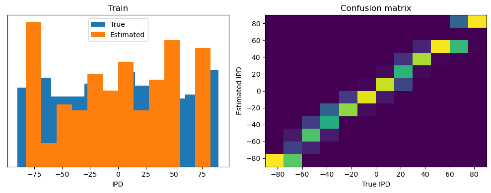
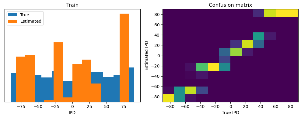
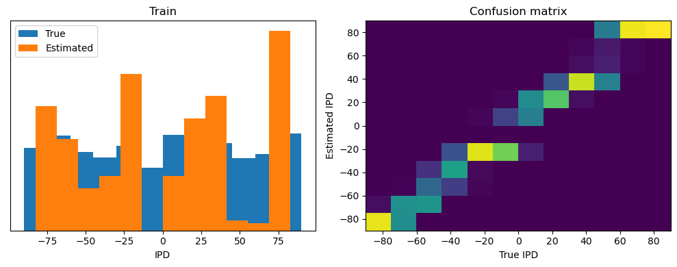
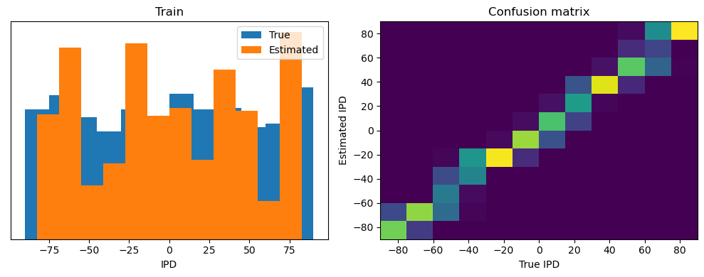

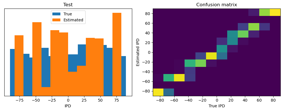
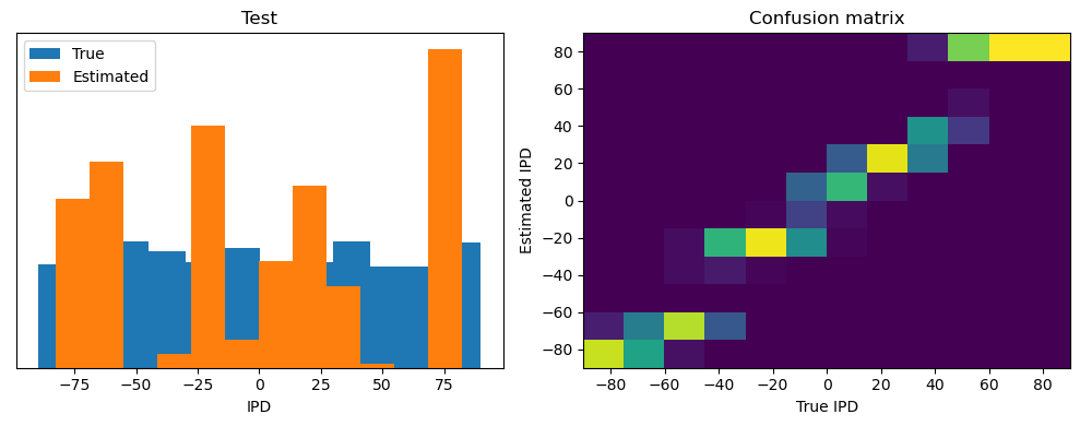
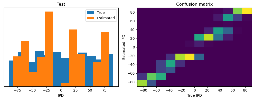
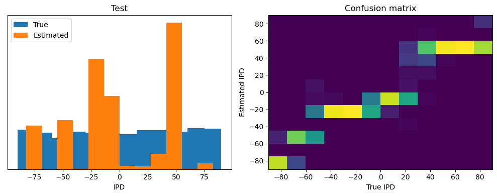
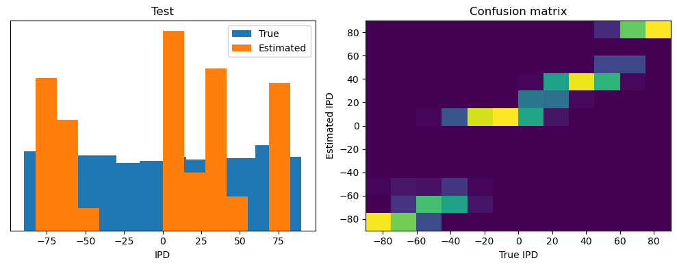
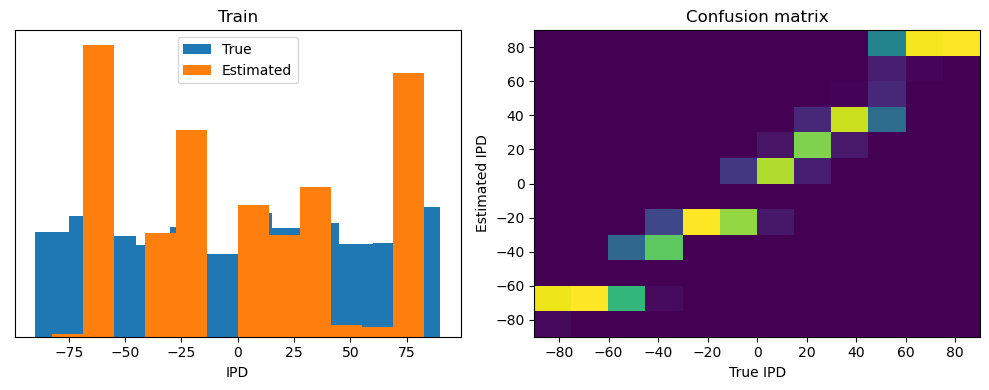
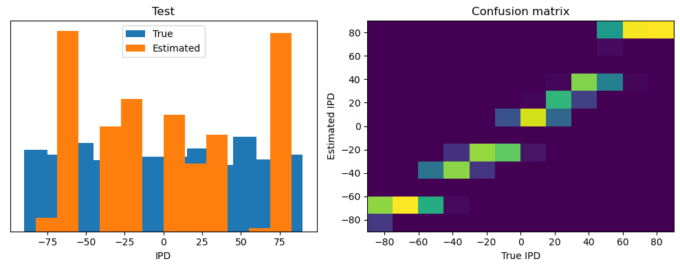
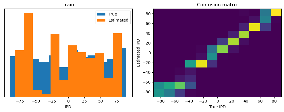
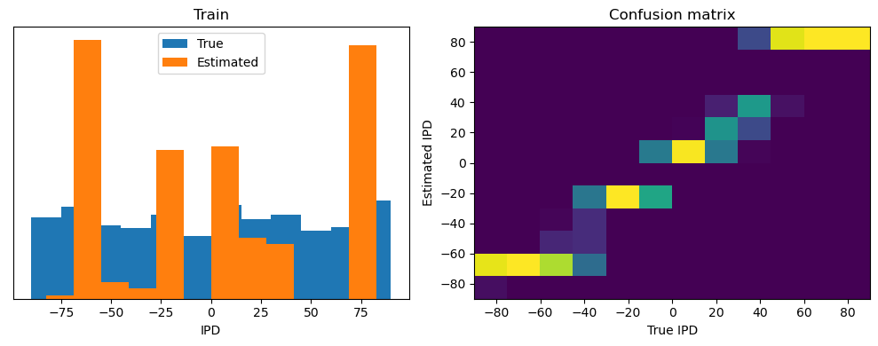
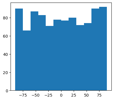
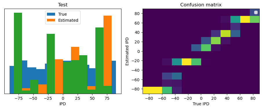
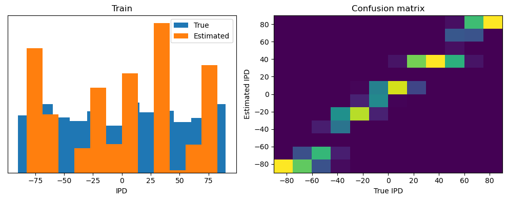
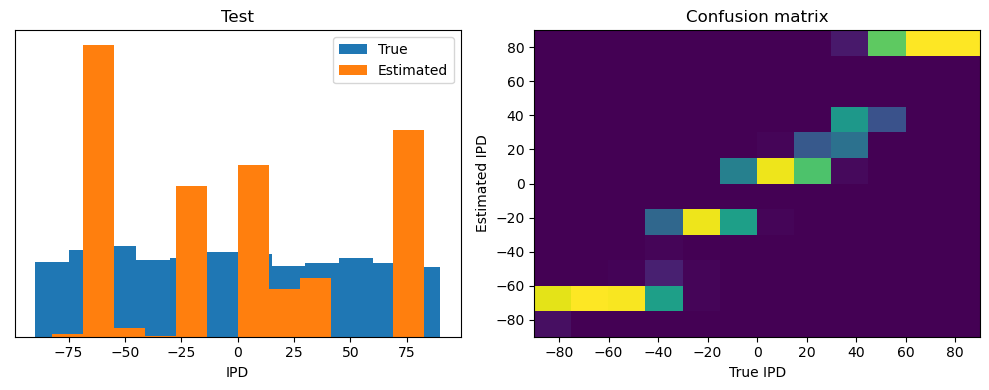
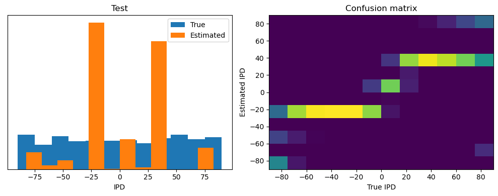
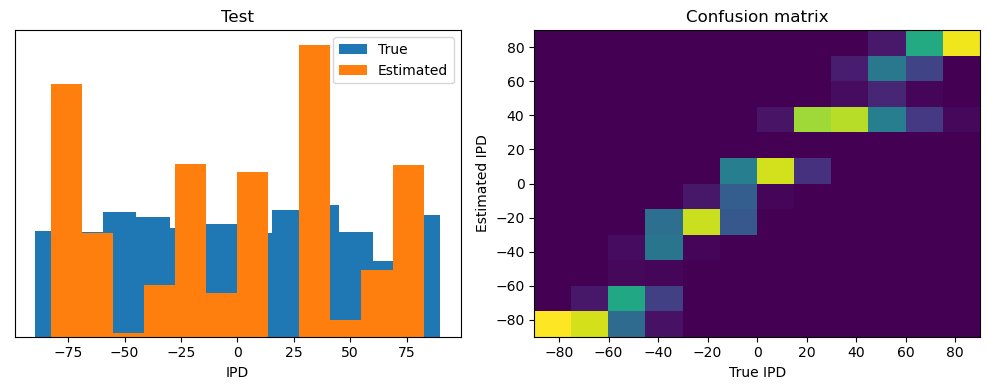
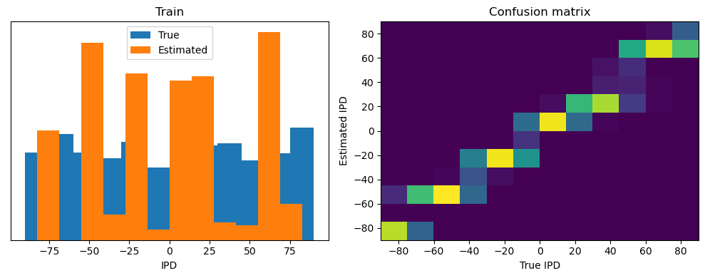
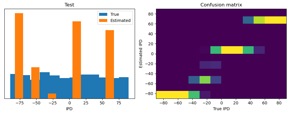
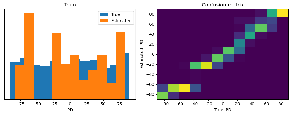
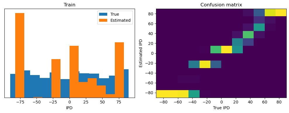
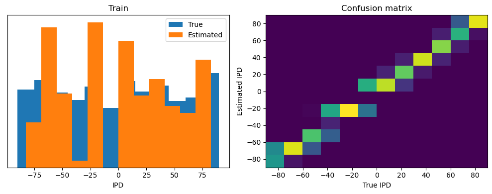
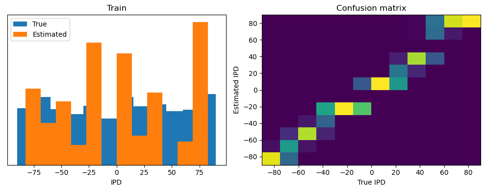
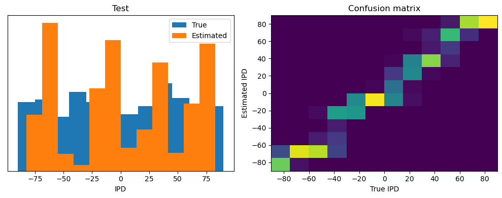
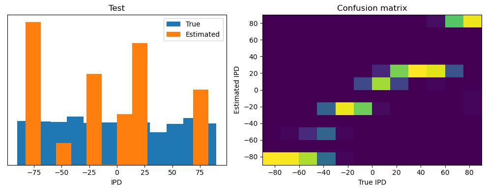
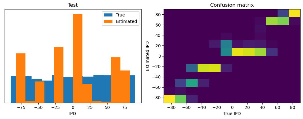
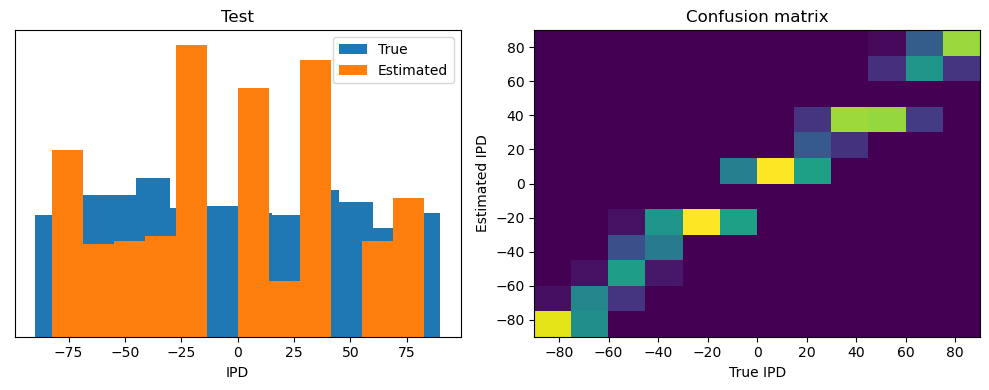
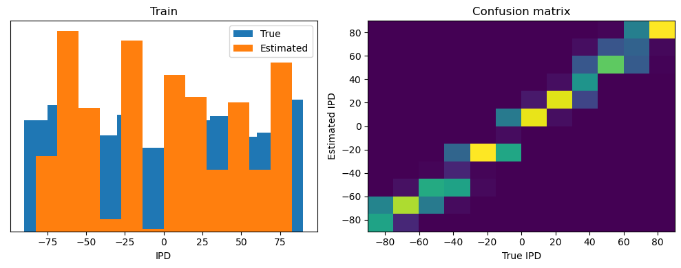
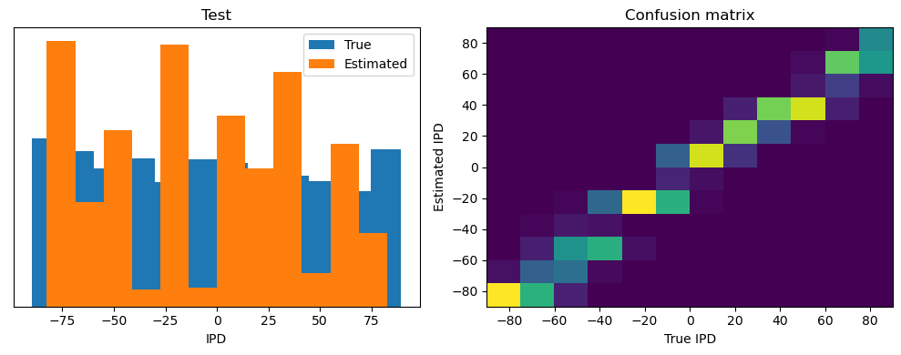
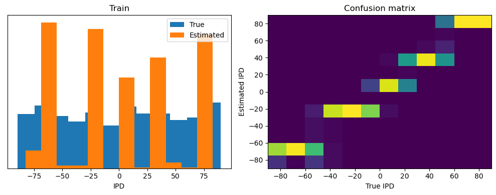
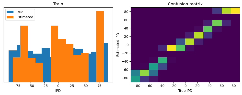
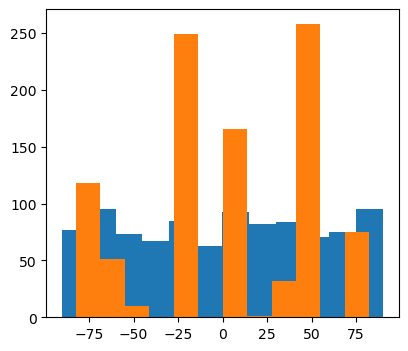
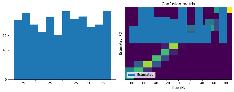
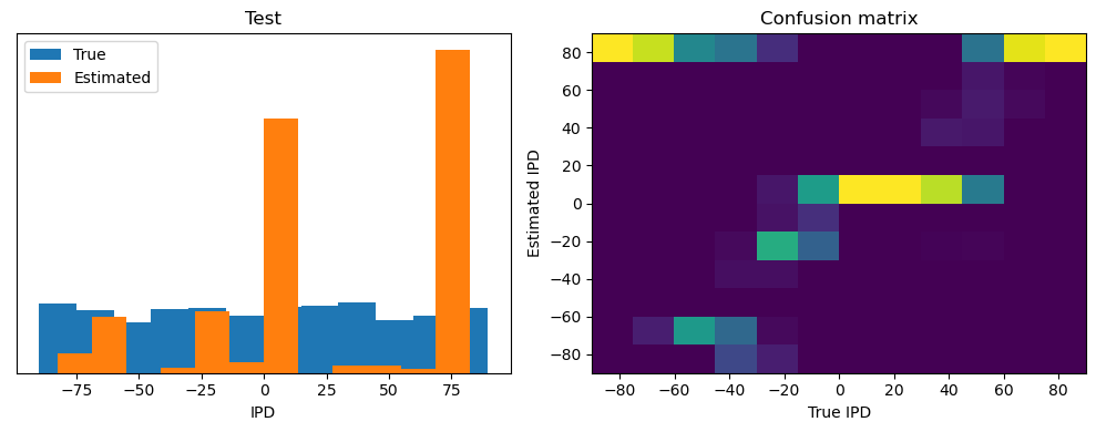
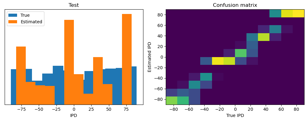
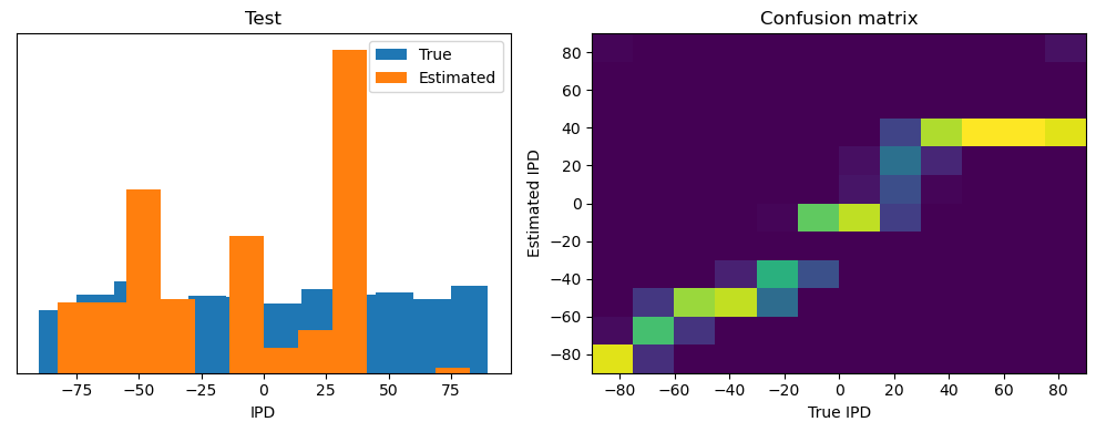
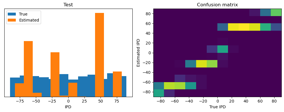
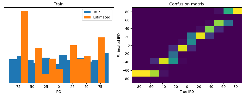
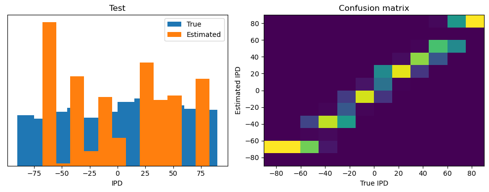
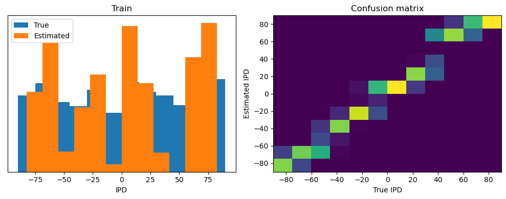
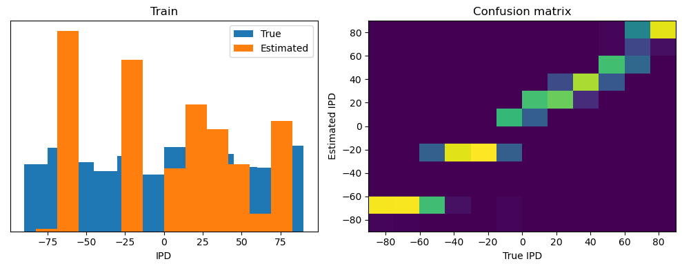
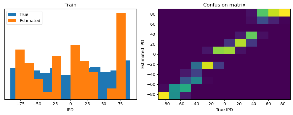
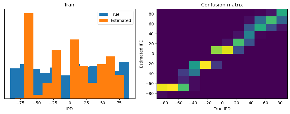
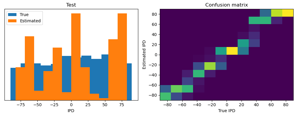
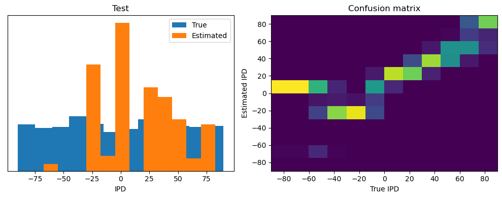
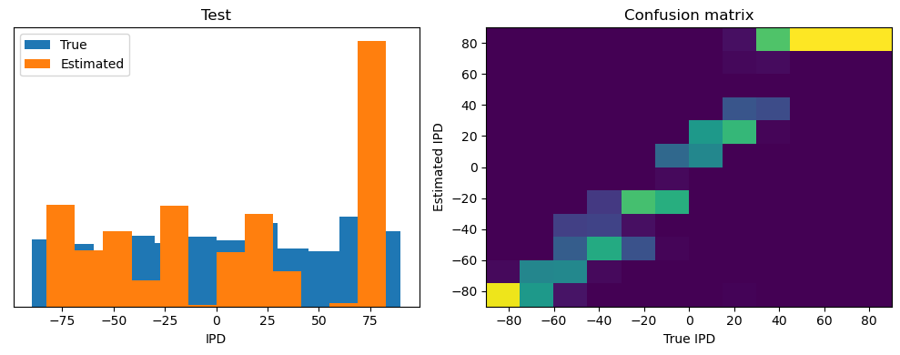
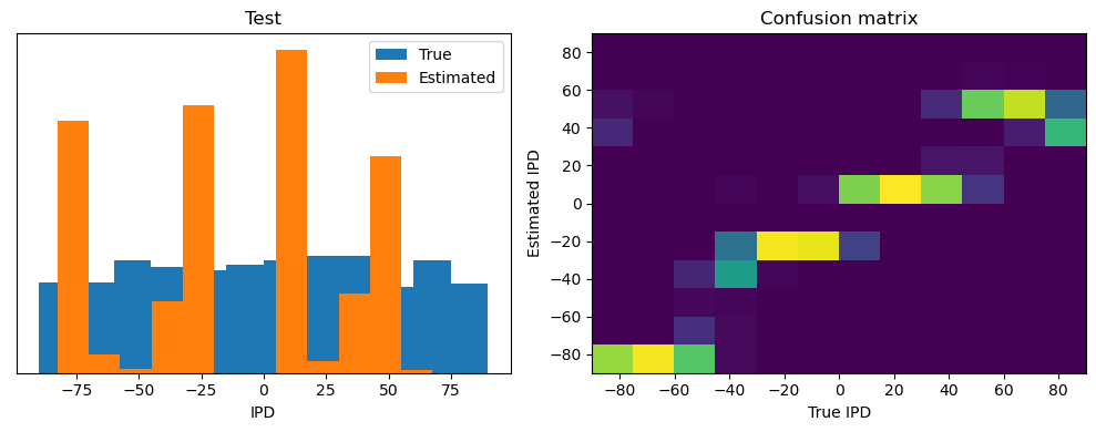
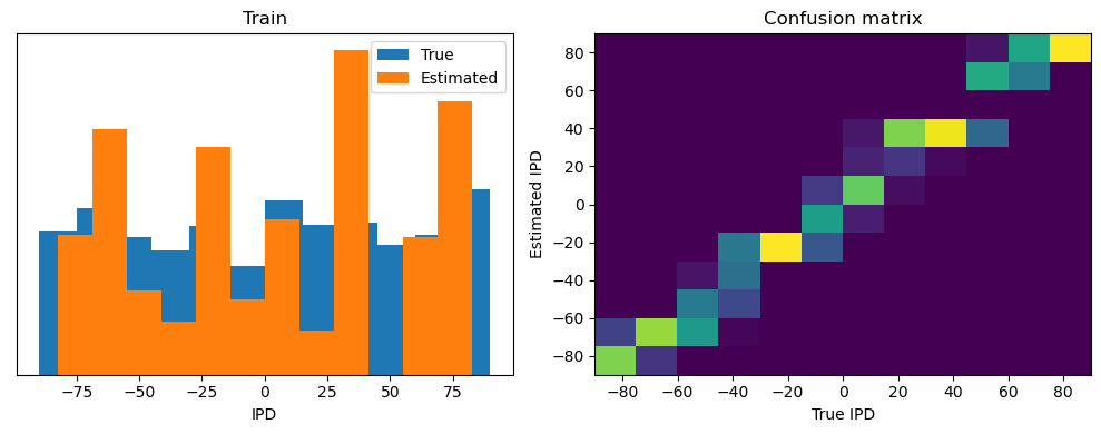
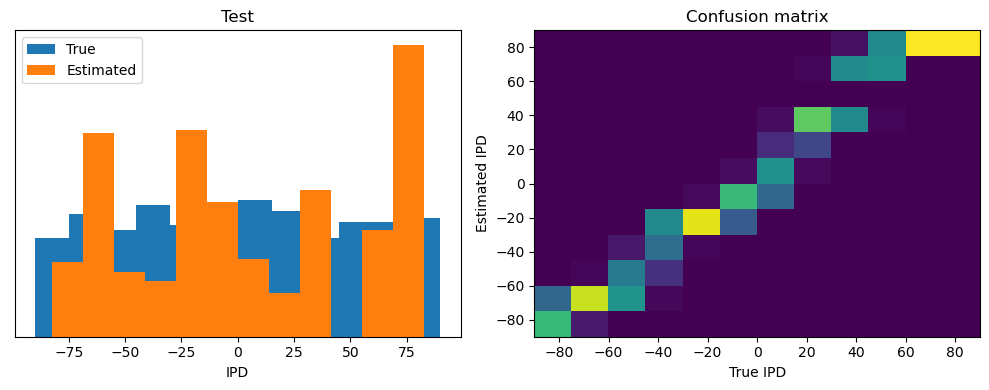

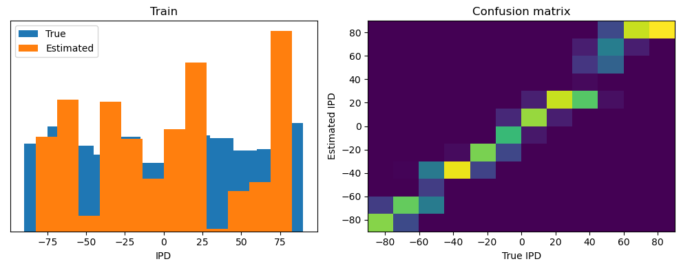
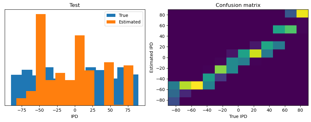
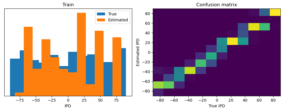
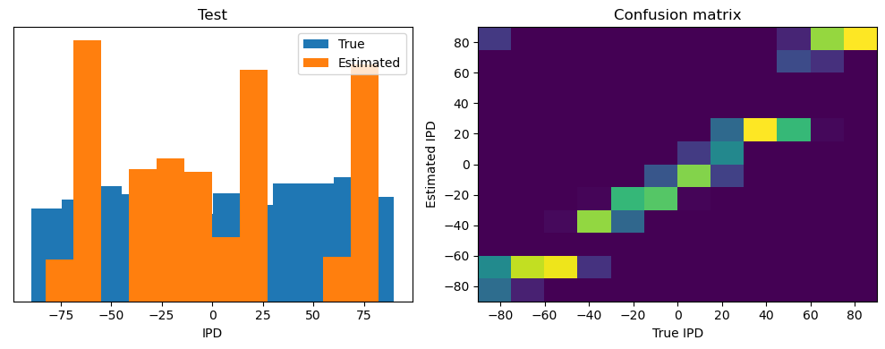
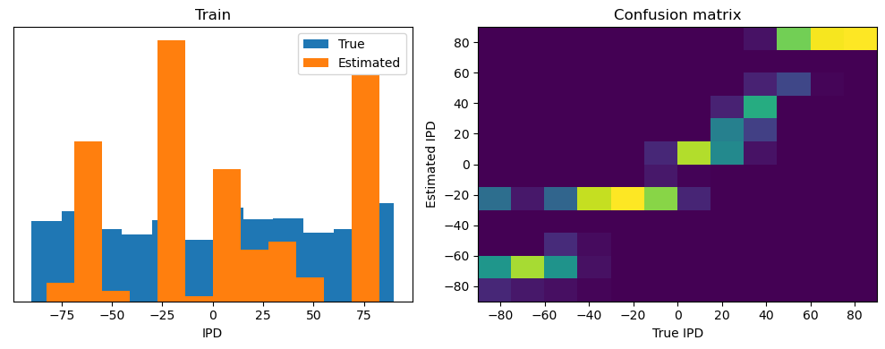
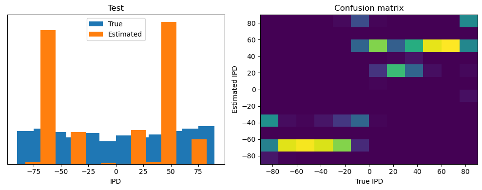
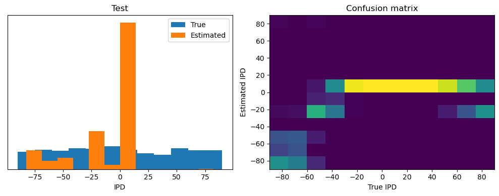
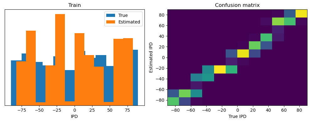
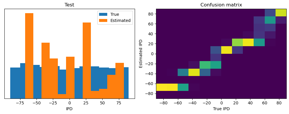
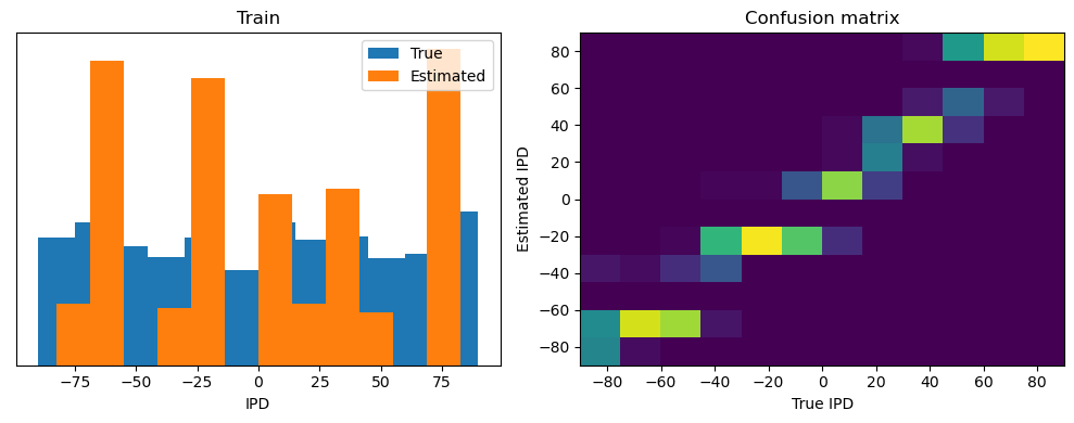
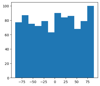
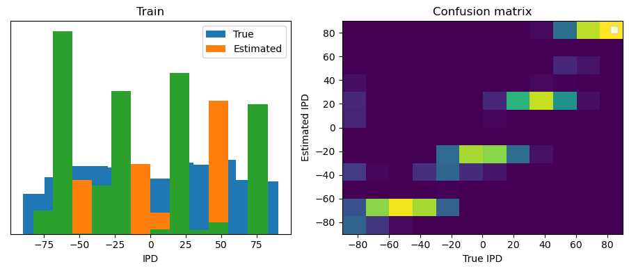
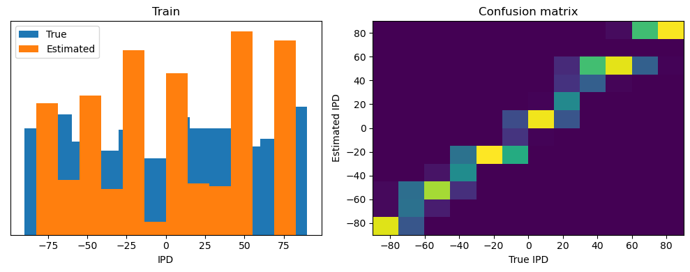
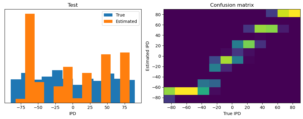
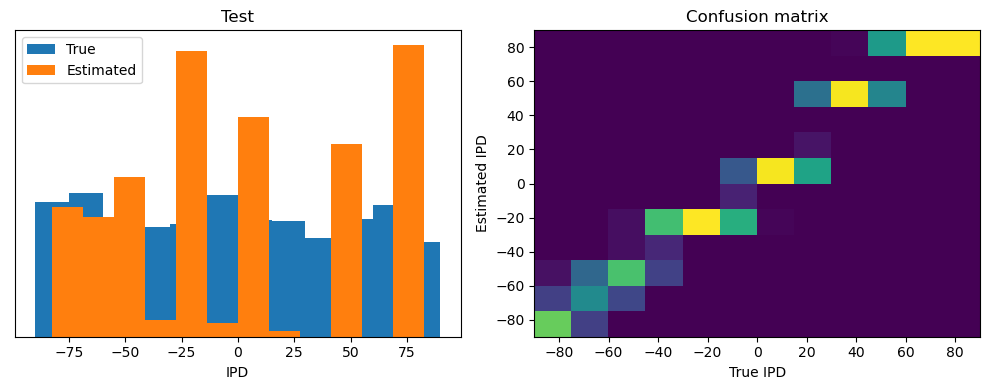
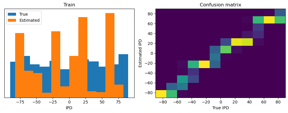
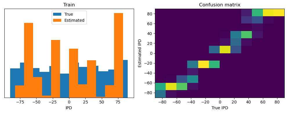
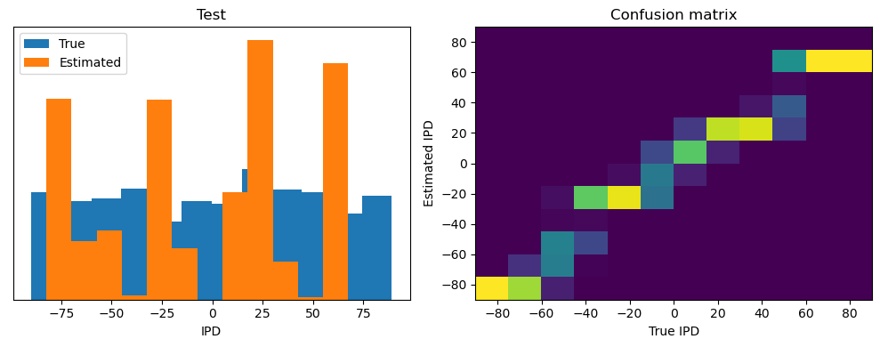
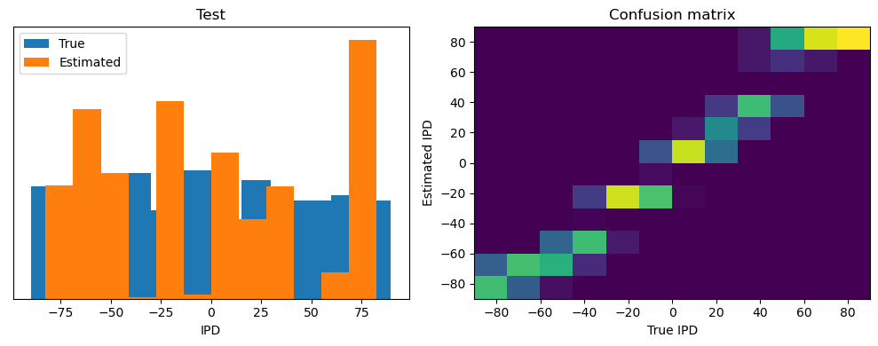
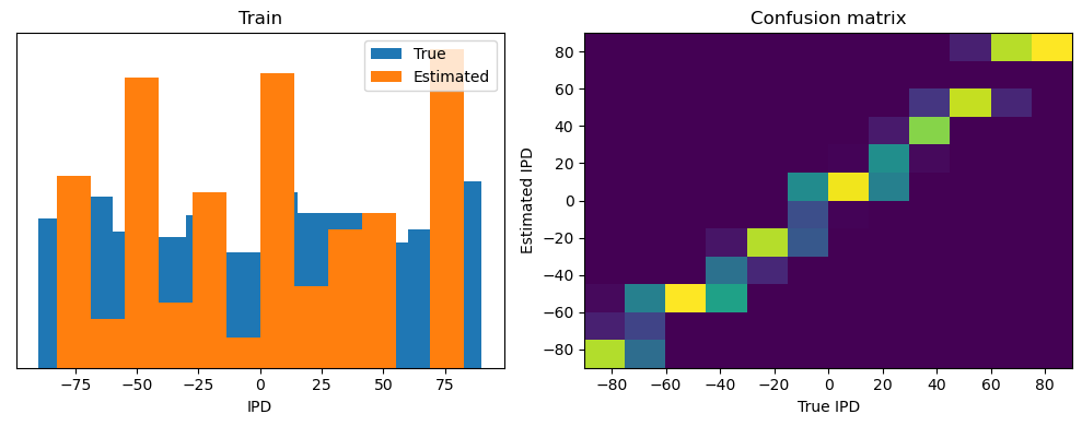
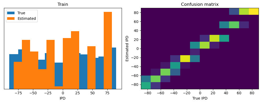
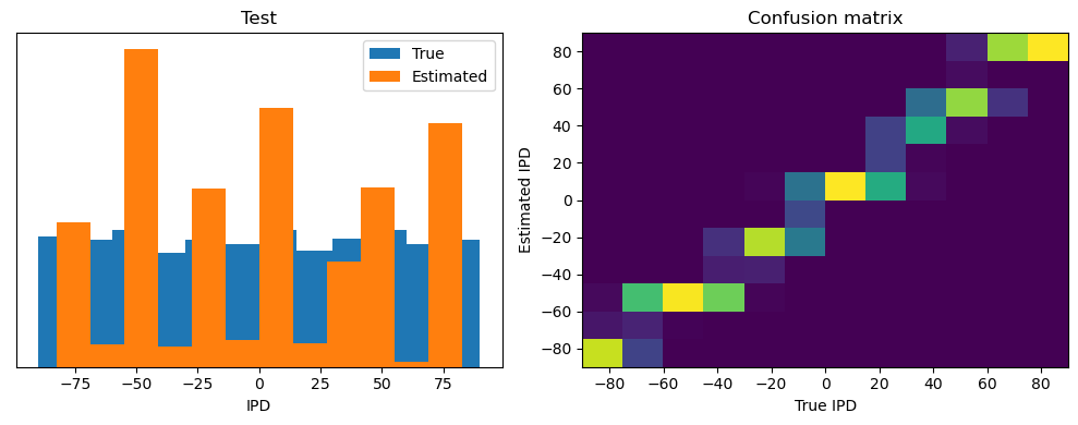
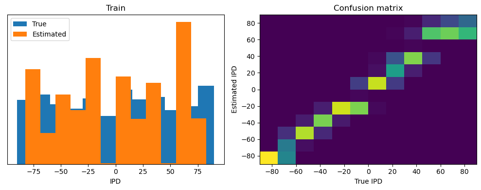
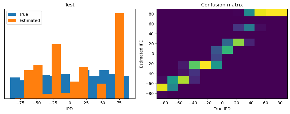
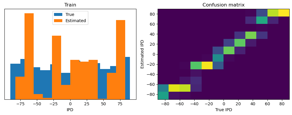
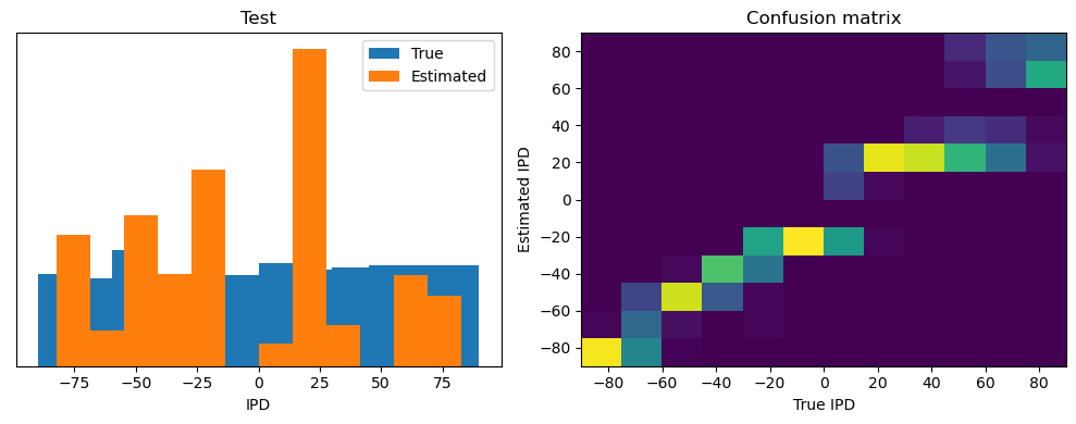
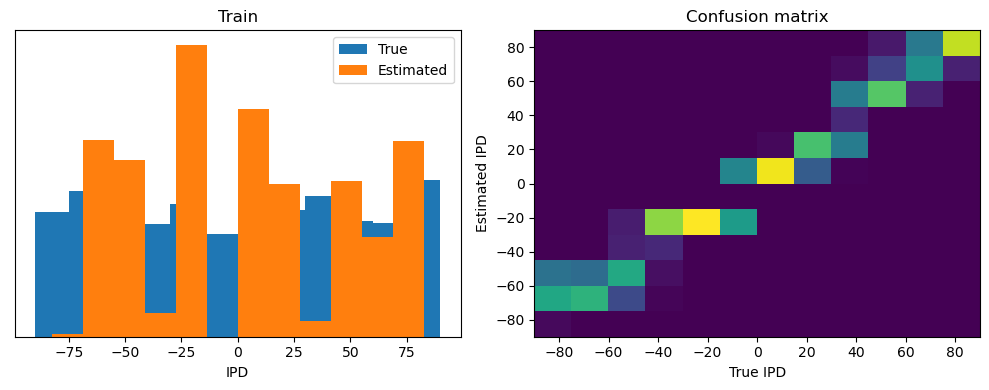
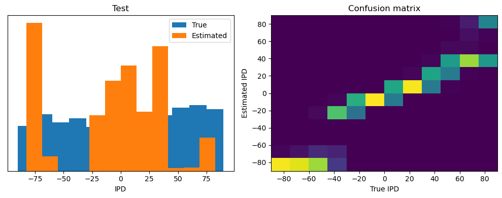
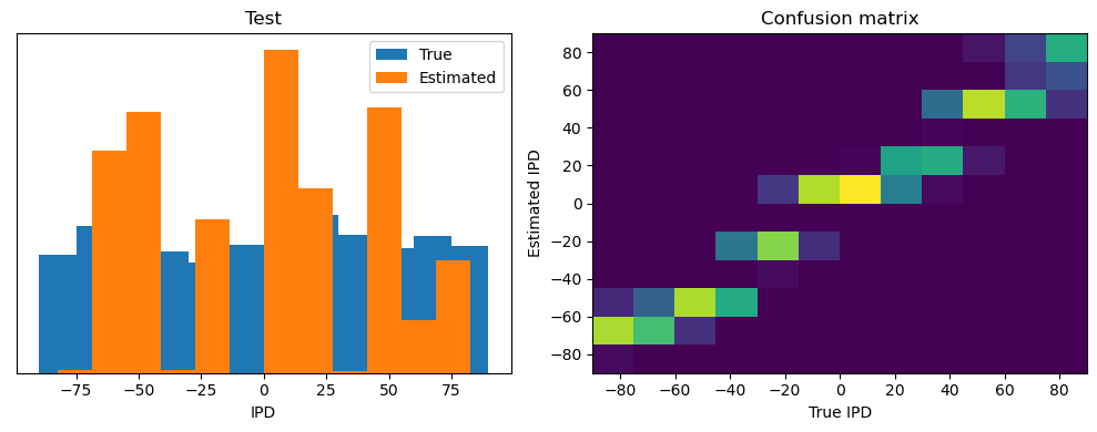
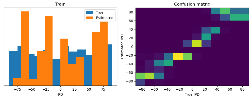
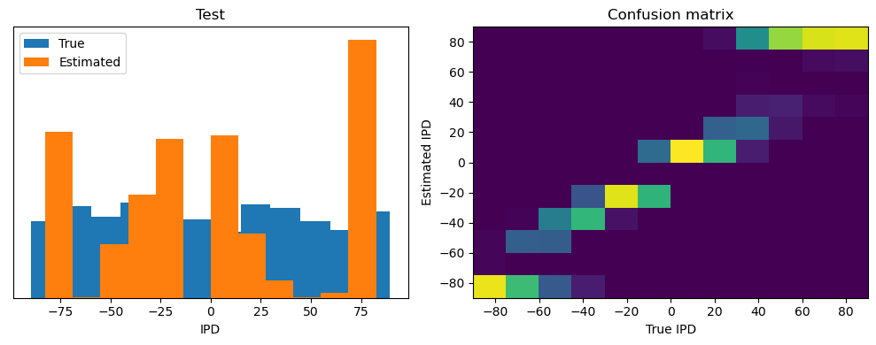
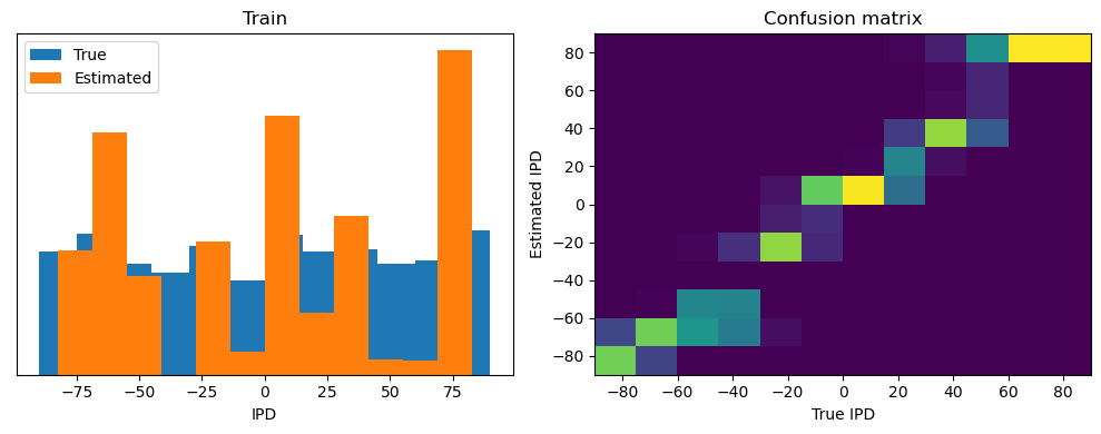
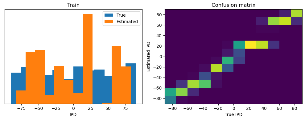
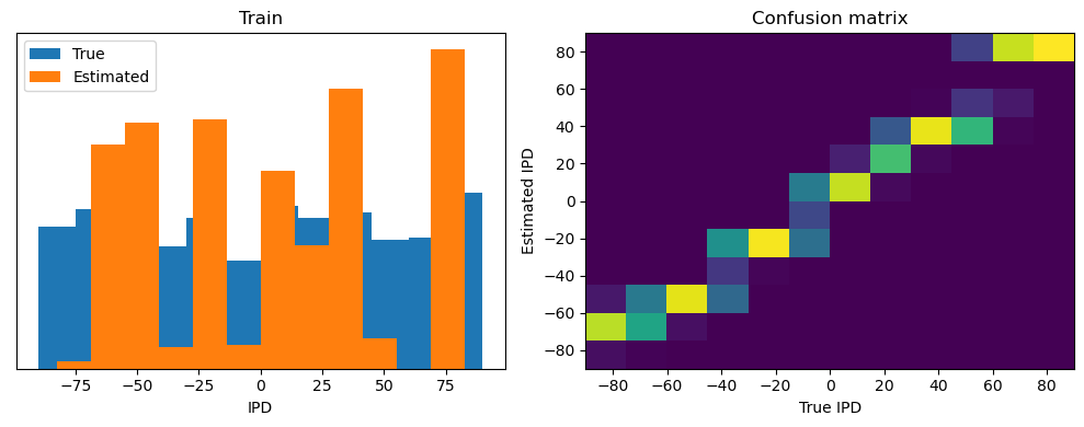
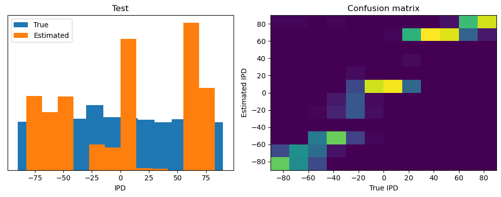
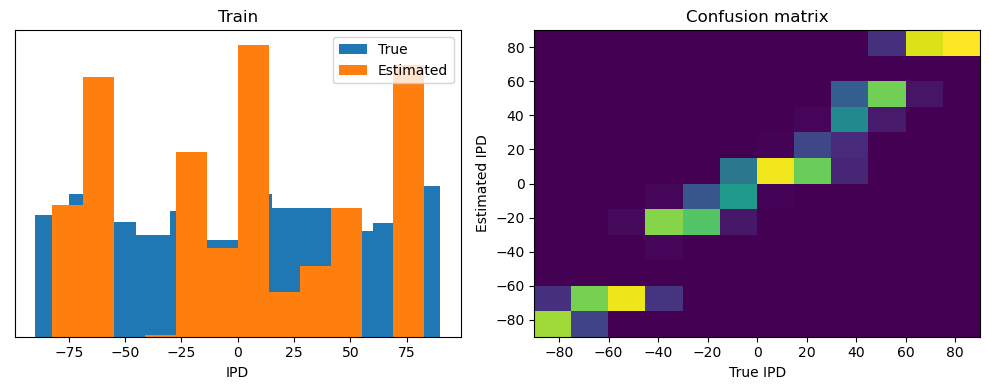
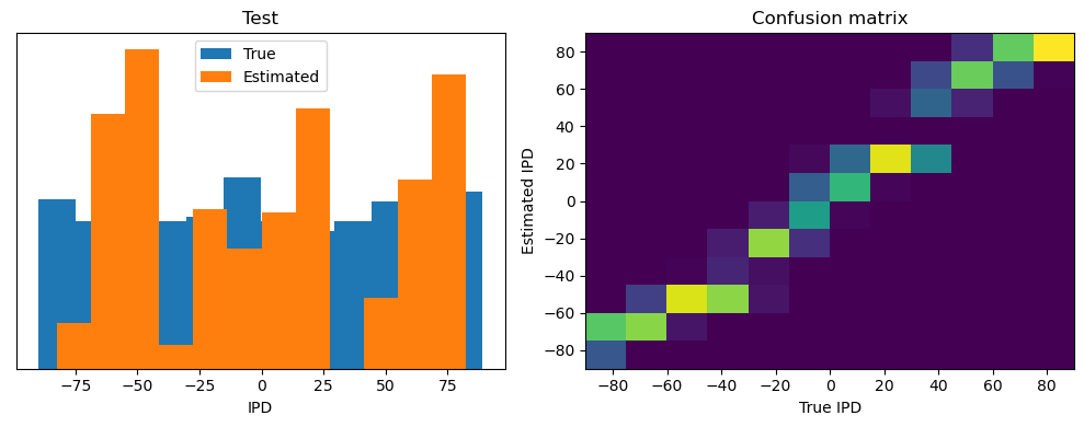
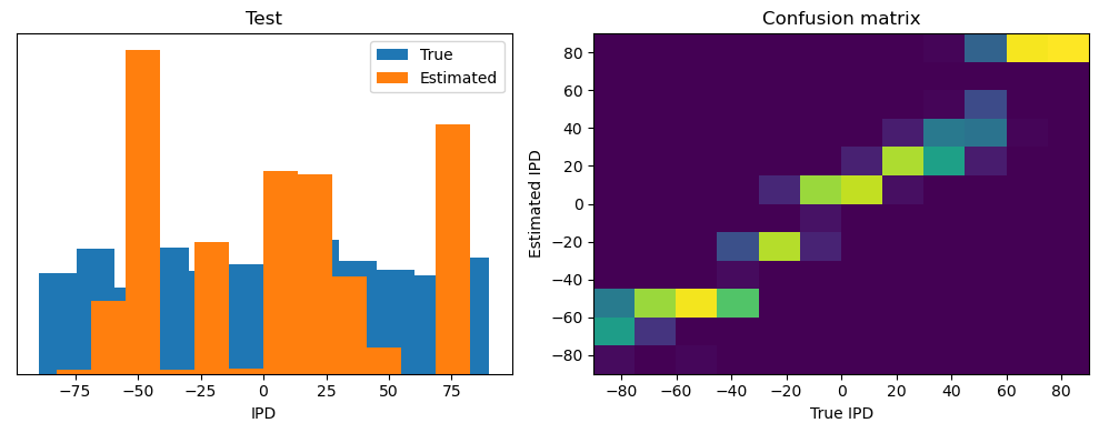
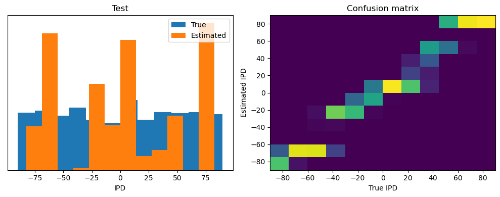
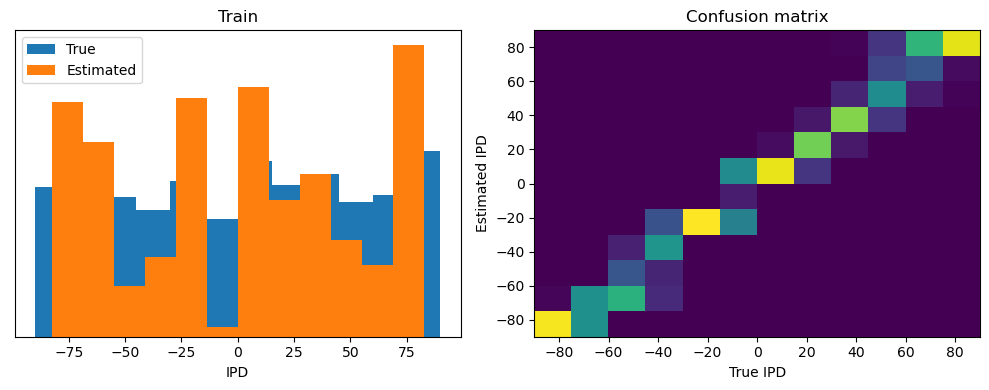
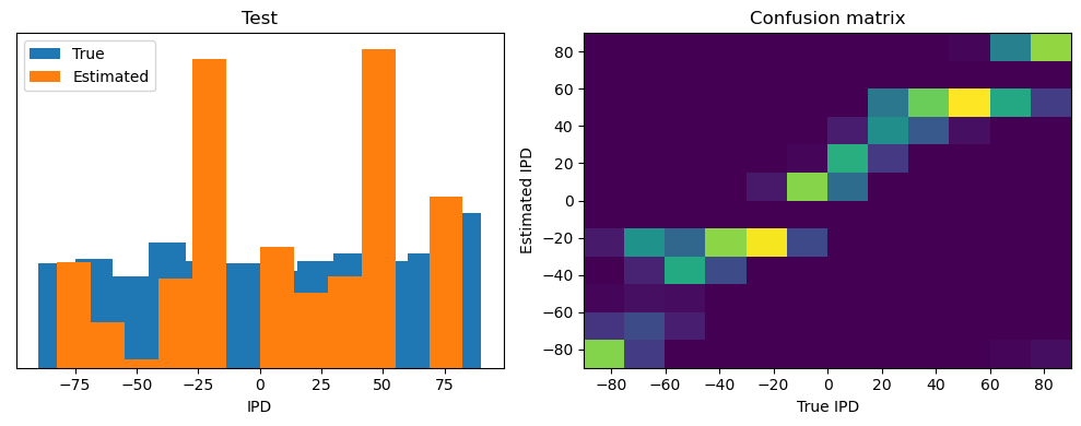
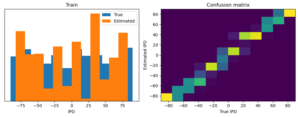
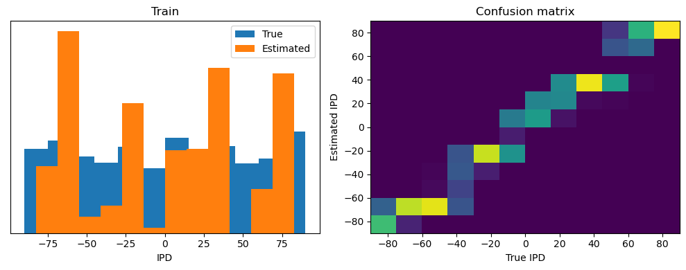
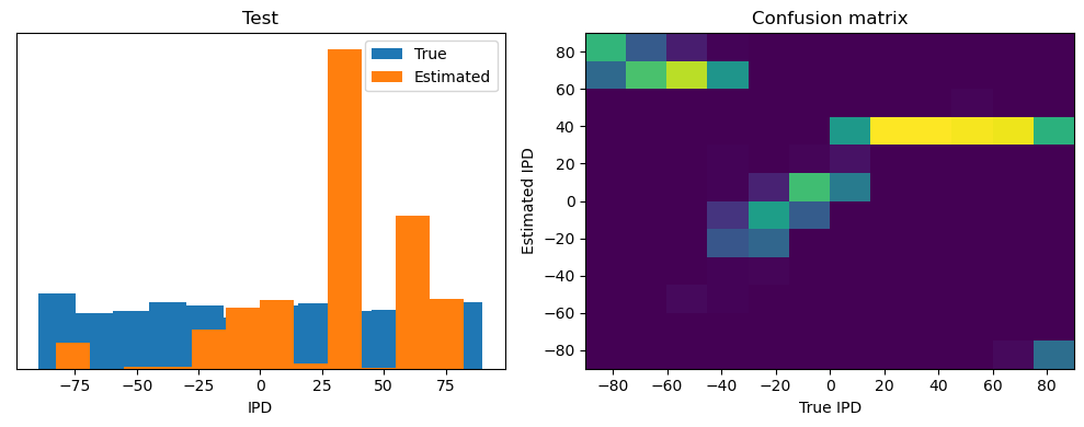
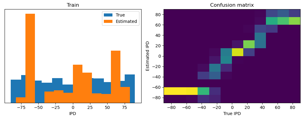
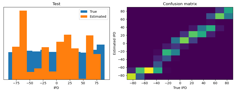
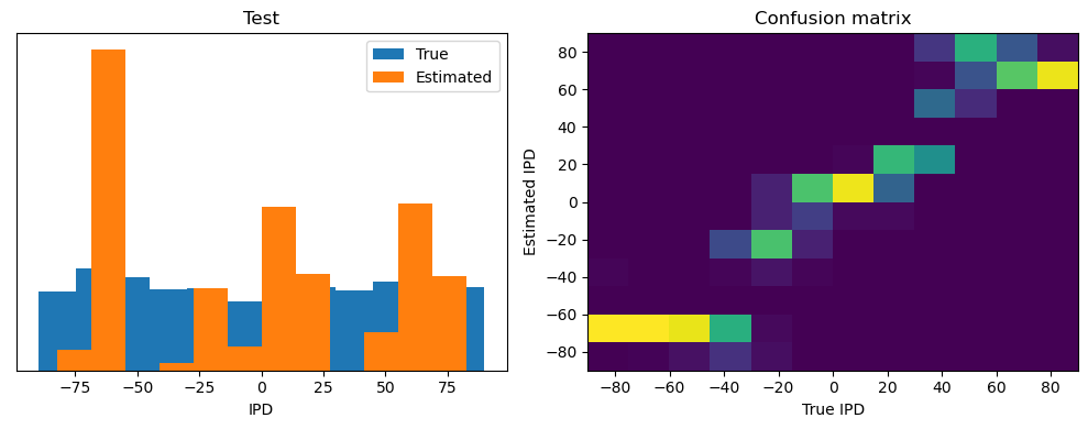
# results[0][0].factors[0].shape  # trial factors
# # results[0][0].factors[1].shape # neuron factors
# # results[0][0].factors[2].shape # time factors

# models = [result[0] for result in results]
# Extracting only the during training models for analysis
models = [result[0] for result in results]
if models:
print("Shape of trial factors:", models[0].factors[0].shape) # trial factors
print("Shape of neuron factors:", models[0].factors[1].shape) # neuron factors
print("Shape of time factors:", models[0].factors[2].shape) # time factorsShape of trial factors: (1, 20)
Shape of neuron factors: (1, 30)
Shape of time factors: (1, 100)
def normalize_data(data):
    return (data - np.min(data)) / (np.max(data) - np.min(data))


def plot_factors(models, normalize_temporal=False):
    fig, axes = plt.subplots(1, 3, figsize=(18, 4))

    temporal_data_all = []

    for i, model in enumerate(models):
        color = plt.cm.viridis(i / len(models))

        # Normalize trial data
        trial_data = normalize_data(model.factors[0][0, :])
        axes[0].plot(trial_data, label=f"Model {i+1}", color=color)

        # Normalize neuron data
        neuron_data = normalize_data(model.factors[1][0, :])
        axes[1].bar(
            np.arange(len(neuron_data)),
            neuron_data,
            label=f"Model {i+1}",
            color=color,
            alpha=0.6,
        )

        # temporal data
        temporal_data = model.factors[2][0, :]
        if normalize_temporal:
            temporal_data = normalize_data(temporal_data)
        axes[2].plot(temporal_data, label=f"Model {i+1}", color=color)

        # shading
        temporal_data_all.append(temporal_data)

    temporal_mean = np.mean(temporal_data_all, axis=0)
    temporal_std = np.std(temporal_data_all, axis=0)

    axes[2].fill_between(
        range(len(temporal_mean)),
        temporal_mean - temporal_std,
        temporal_mean + temporal_std,
        color="gray",
        alpha=0.3,
    )

    axes[0].set_title("Normalized Trial Factors")
    axes[1].set_title("Normalized Neuron Factors (Bar)")
    axes[2].set_title("Temporal Factors with Shading")

    # for ax in axes:
    #     ax.legend(loc="upper right")
    # ax.grid(True)

    plt.tight_layout()
    # plt.show()


plot_factors(models, normalize_temporal=True)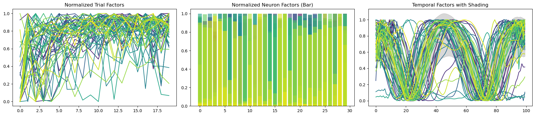
def plot_temporal_factors(models, normalize_temporal=False):
    fig, ax = plt.subplots(figsize=(10, 5))

    temporal_data_all = []

    for i, model in enumerate(models):
        color = plt.cm.viridis(i / len(models))

        temporal_data = model.factors[2][0, :]
        if normalize_temporal:
            temporal_data = normalize_data(temporal_data)
        ax.plot(temporal_data, label=f"Model {i+1}", color=color, alpha=0.4)

        temporal_data_all.append(temporal_data)

    temporal_mean = np.mean(temporal_data_all, axis=0)
    temporal_std = np.std(temporal_data_all, axis=0)

    ax.fill_between(
        range(len(temporal_mean)),
        temporal_mean - temporal_std,
        temporal_mean + temporal_std,
        color="gray",
        alpha=0.5,
    )

    # ax.set_title("Temporal Factors with Shading")
    ax.set_xlabel("Time Step")
    ax.set_ylabel("Activation")

    # if len(models) > 1:
    #     ax.legend(loc="upper right")
    ax.grid(True)

    plt.tight_layout()
    # plt.show()


plot_temporal_factors(models, normalize_temporal=True)
plt.savefig(str(fig_counter) + '.png', dpi=300)
plt.savefig(str(fig_counter) + '.tiff', dpi=300)
fig_counter += 1
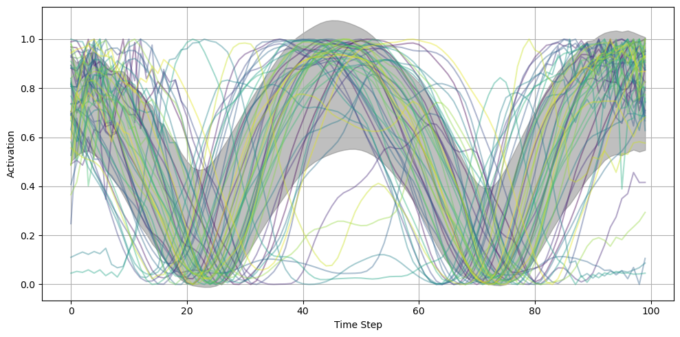
from sklearn.preprocessing import StandardScaler
from scipy.cluster.hierarchy import dendrogram, linkage, fcluster


def normalize_data(data):
    """Normalize the data to have zero mean and unit variance."""
    scaler = StandardScaler()
    data = data.reshape(-1, 1)  # Reshape data to 2D if it's 1D
    normalized_data = scaler.fit_transform(data)
    return normalized_data.flatten()


sorted_normalized_factors = []
for model in models:
    normalized_factors = normalize_data(model.factors[1][0, :])
    indices = np.argsort(normalized_factors)[::-1]  # Sort by descending order
    sorted_factors = normalized_factors[indices]
    sorted_normalized_factors.append(sorted_factors)

neuron_factors = np.vstack(sorted_normalized_factors)
Z = linkage(neuron_factors, method="ward")

# Determine the clusters at a certain distance threshold
cluster_labels = fcluster(Z, t=5, criterion="distance")
# Count number of models per cluster
cluster_count = np.bincount(cluster_labels)
# Find the most prevalent cluster
most_prevalent_cluster = np.argmax(cluster_count[1:]) + 1

# Filter models that belong to the most prevalent cluster
cluster_models = [
    models[i] for i in range(len(models)) if cluster_labels[i] == most_prevalent_cluster
]

plt.figure(figsize=(10, 7))
dendrogram(
    Z,
    labels=[f"Model {i+1}" for i in range(len(models))],
    leaf_rotation=90,
    leaf_font_size=12,
)
plt.title("Hierarchical Clustering of Sorted Neuron Factors")
plt.xlabel("Model")
plt.ylabel("Distance (Ward's method)")
# plt.show()

plt.savefig(str(fig_counter) + '.png', dpi=300)
plt.savefig(str(fig_counter) + '.tiff', dpi=300)
fig_counter += 1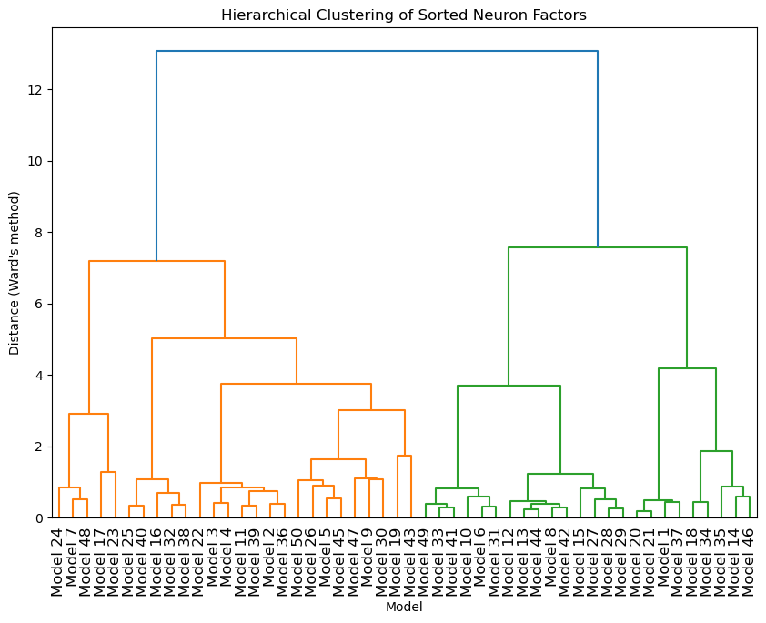
# Plot temporal factors for models in the most prevalent cluster
plot_temporal_factors(cluster_models, normalize_temporal=True)

plt.savefig(str(fig_counter) + '.png', dpi=300)
plt.savefig(str(fig_counter) + '.tiff', dpi=300)
fig_counter += 1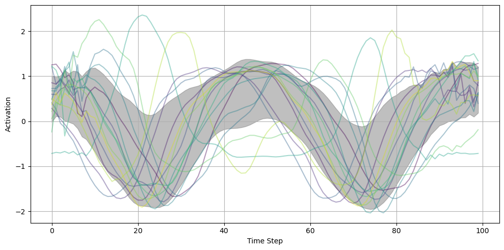
def count_highly_active_neurons(neuron_factors, threshold=0.5):
    """Count the number of neurons that are above the activation threshold."""
    return (neuron_factors > threshold).sum(axis=1)


# Normalize and sort the neuron factors
sorted_normalized_neurons = []
for model in models:
    normalized_neurons = normalize_data(model.factors[1][0, :])
    sorted_neurons = np.sort(normalized_neurons)[::-1]
    sorted_normalized_neurons.append(sorted_neurons)

# Stack and cluster
neuron_factors = np.vstack(sorted_normalized_neurons)
Z = linkage(neuron_factors, method="ward")
cluster_labels = fcluster(Z, t=5, criterion="distance")

# Analyze clusters
cluster_stats = {}
for cluster_label in np.unique(cluster_labels):
    indices = np.where(cluster_labels == cluster_label)[0]
    cluster_neurons = neuron_factors[indices]
    active_counts = count_highly_active_neurons(cluster_neurons)
    train_accuracies = [accuracies.iloc[i]["Train Accuracy"] for i in indices]
    test_accuracies = [accuracies.iloc[i]["Test Accuracy"] for i in indices]
    cluster_stats[cluster_label] = {
        "models": indices,
        "active_neuron_counts": active_counts,
        "average_active_neurons": np.mean(active_counts),
        "std_dev_active_neurons": np.std(active_counts),
        "average_train_accuracy": np.mean(train_accuracies),
        "average_test_accuracy": np.mean(test_accuracies),
        "train_accuracies": accuracies.iloc[indices]["Train Accuracy"].values,
        "test_accuracies": accuracies.iloc[indices]["Test Accuracy"].values,
    }

# Output the results for analysis
for label, stats in cluster_stats.items():
    print(f"Cluster {label}:")
    print(f"  Number of models: {len(stats['models'])}")
    print(f"  Average highly active neurons: {stats['average_active_neurons']:.2f}")
    print(f"  Standard deviation: {stats['std_dev_active_neurons']:.2f}")
    print(f"  Average Train Accuracy: {stats['average_train_accuracy']:.2f}%")
    print(f"  Average Test Accuracy: {stats['average_test_accuracy']:.2f}%")
    print(f"  Active counts per model: {stats['active_neuron_counts']}")
Cluster 1:
Number of models: 5
Average highly active neurons: 4.20
Standard deviation: 1.60
Average Train Accuracy: 57.52%
Average Test Accuracy: 29.77%
Active counts per model: [6 2 3 4 6]
Cluster 2:
Number of models: 5
Average highly active neurons: 3.40
Standard deviation: 0.80
Average Train Accuracy: 59.85%
Average Test Accuracy: 36.42%
Active counts per model: [5 3 3 3 3]
Cluster 3:
Number of models: 16
Average highly active neurons: 4.81
Standard deviation: 0.81
Average Train Accuracy: 57.53%
Average Test Accuracy: 39.22%
Active counts per model: [5 5 5 4 4 5 5 5 4 4 5 5 7 4 6 4]
Cluster 4:
Number of models: 15
Average highly active neurons: 6.47
Standard deviation: 0.50
Average Train Accuracy: 57.26%
Average Test Accuracy: 45.95%
Active counts per model: [7 6 7 6 6 7 6 6 6 7 7 7 6 6 7]
Cluster 5:
Number of models: 9
Average highly active neurons: 9.67
Standard deviation: 1.25
Average Train Accuracy: 62.33%
Average Test Accuracy: 50.57%
Active counts per model: [11 9 8 11 11 8 9 11 9]
New plot
fig, ax = plt.subplots(figsize=(10, 6))
positions = np.arange(len(cluster_stats))

# Sort clusters based on average active neurons
sorted_clusters = sorted(
    cluster_stats.items(), key=lambda x: x[1]["average_active_neurons"]
)

# Plot train and test accuracies for each cluster
for i, (cluster, stats) in enumerate(sorted_clusters):
    train_accuracies = stats["train_accuracies"]
    test_accuracies = stats["test_accuracies"]

    jitter = np.random.normal(0, 0.05, size=len(train_accuracies))  # Reduced jitter

    # training accuracies
    ax.scatter(
        positions[i] + jitter - 0.15,
        train_accuracies,
        color="dodgerblue",
        s=50,
        alpha=0.7,
        marker="o",
        edgecolors="black",
        label="Train Accuracy" if i == 0 else "",
    )

    # testing accuracies
    ax.scatter(
        positions[i] + jitter + 0.15,
        test_accuracies,
        color="limegreen",
        s=50,
        alpha=0.7,
        marker="s",
        edgecolors="black",
        label="Test Accuracy" if i == 0 else "",
    )

    # median values with a line
    median_train = np.median(train_accuracies)
    median_test = np.median(test_accuracies)
    ax.plot(
        [positions[i] - 0.15, positions[i] + 0.15],
        [median_train, median_test],
        "k-",
        alpha=0.75,
        marker="o",
        markersize=8,
    )

# Styling
ax.set_xticks(positions)
ax.set_xticklabels([f"Cluster {cluster}" for cluster in cluster_stats.keys()])
# ax.set_xticklabels([f"Cluster {cluster}" for cluster, _ in sorted_clusters])
ax.set_ylabel("Accuracy (%)")
# ax.set_title("Training and Test Accuracies by Cluster")
ax.legend()
ax.grid(True)

plt.tight_layout()
# plt.show()

plt.savefig(str(fig_counter) + '.png', dpi=300)
plt.savefig(str(fig_counter) + '.tiff', dpi=300)
fig_counter += 1